Now that we know how to create a 3×3 linear matrix to convert white balanced and demosaiced raw data into  connection space – and where to obtain the 3×3 linear matrix to then convert it to a standard output color space like sRGB – we can take a closer look at the matrices and apply them to a real world capture chosen for its wide range of chromaticities.

The Forward Matrix Analyzed

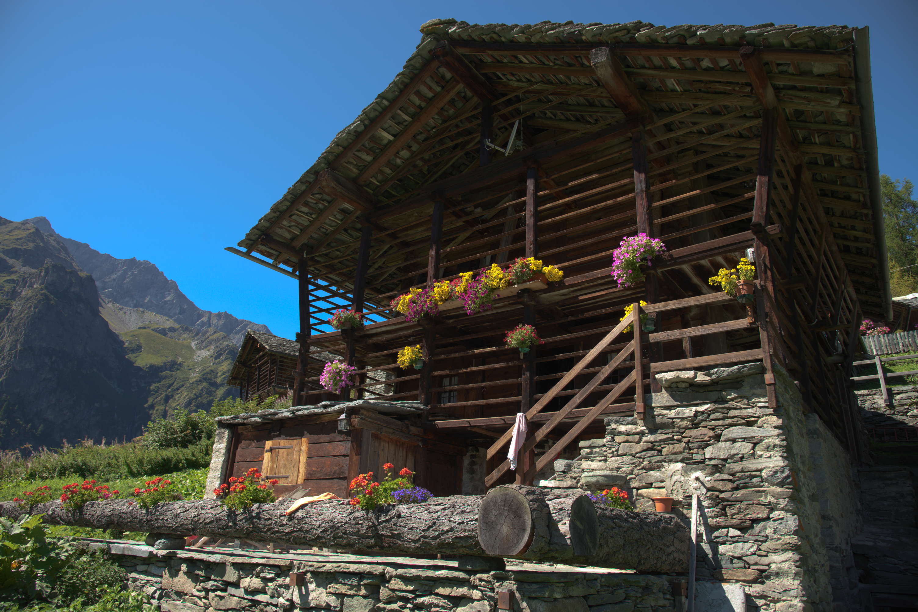
I captured a ColorChecker Passport Photo 24 patch target shortly after squeezing the trigger on the scene depicted in Figure 1, with a Nikon D610 and Nikkor 24-120mm f/4 at base ISO.  The time was about 1:15pm of a clear, late summer day in the Alps at an altitude of 1600m, so I assumed the illuminant to be fairly close to D50 ‘daylight’.  Let’s assume that’s the case, though it turns out that Correlated Color Temperature at the time of taking was actually around 5350K.

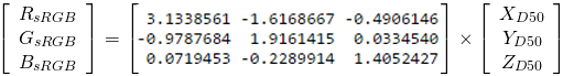
I then followed the procedure outlined in the last article to obtain the linear matrix needed to convert white balanced and minimally demosaiced raw data^[2] – indicated as in this article – into CIE Profile Connection Space with the given illuminant:

The Forward Matrix is applied to every pixel by matrix multiplication as follows:

   

Note that the matrix contains some negative coefficients, which are larger in the Y and Z rows.   However, RGB values from the camera can only be positive and XYZ  primaries were chosen specifically so that visible colors would only have positive values within the space.  This means that after multiplication by the Forward Matrix some  values captured in the raw data could  turn out to be substantially negative in Y or Z, falling outside of the visible realm.  With the given compromise matrix such tones would be out of gamut as captured, more on this around Figure 4 below.

The sum of the coefficients of each row shown at the bottom of Figure 2 are the XYZ values that will be obtained when the  input is [1 1 1], that is from a properly white balanced neutral white patch of demosaiced raw data.  Since the reference values of the target used to estimate the matrix are for illuminant D50, the result with unity input  should therefore represent the coordinates of D50 in XYZ space, its so-called White Point.  A quick check with Bruce Lindbloom’s calculator^[3] shows indeed a correlated color temperature of 5003.8K at the  shown [0.9613  1.0000  0.8193] XYZ coordinates. The matrix is doing its job properly.

The second row of the Forward Matrix produces the Y values , which are supposed to be proportional  to photometric Luminance.  Note that its coefficients add to 1.000 by design in order not to vary the luminance of the resulting image, potentially reducing the number of unknown matrix coefficients from 9 to 8 (right?).

In fact, a non-neutral Forward Matrix (i.e. one with the sum of the rows substantially different from the White Point of the illuminant) can result in objectionable color casts.  Since to do a decent job of finding the optimum compromise color matrix we need to know the illuminant and its CCT or White Point anyways, we could decide to force the sum of the rows to be equal to the White Point in XYZ.  This would effectively reduce the number of unknown matrix coefficients from 9 to 6.  In what follows I decided to keep the 9 unknowns to maintain the most degrees of freedom in order to find the best fit possible, while making sure that the matrix’s White Point and luminance gain (k) did not stray too far from expected values, as I did above.

Applying the Forward Matrix

The capture in Figure 1 was exposed ‘properly’ by my standards, with RawDigger reporting less than 2k pixels blown in the R and B raw channels combined and just 7k in the G channels. That’s as captured.  However the white balance multipliers obtained from ColorChecker’s second gray patch from the left were 1.9615 for R and 1.3336 for B, so after white balancing the situation may worsen. Below you can see an animated GIF alternating every 2s of the white balanced raw data before clipping.  You can open it full size in a new tab by clicking on it.

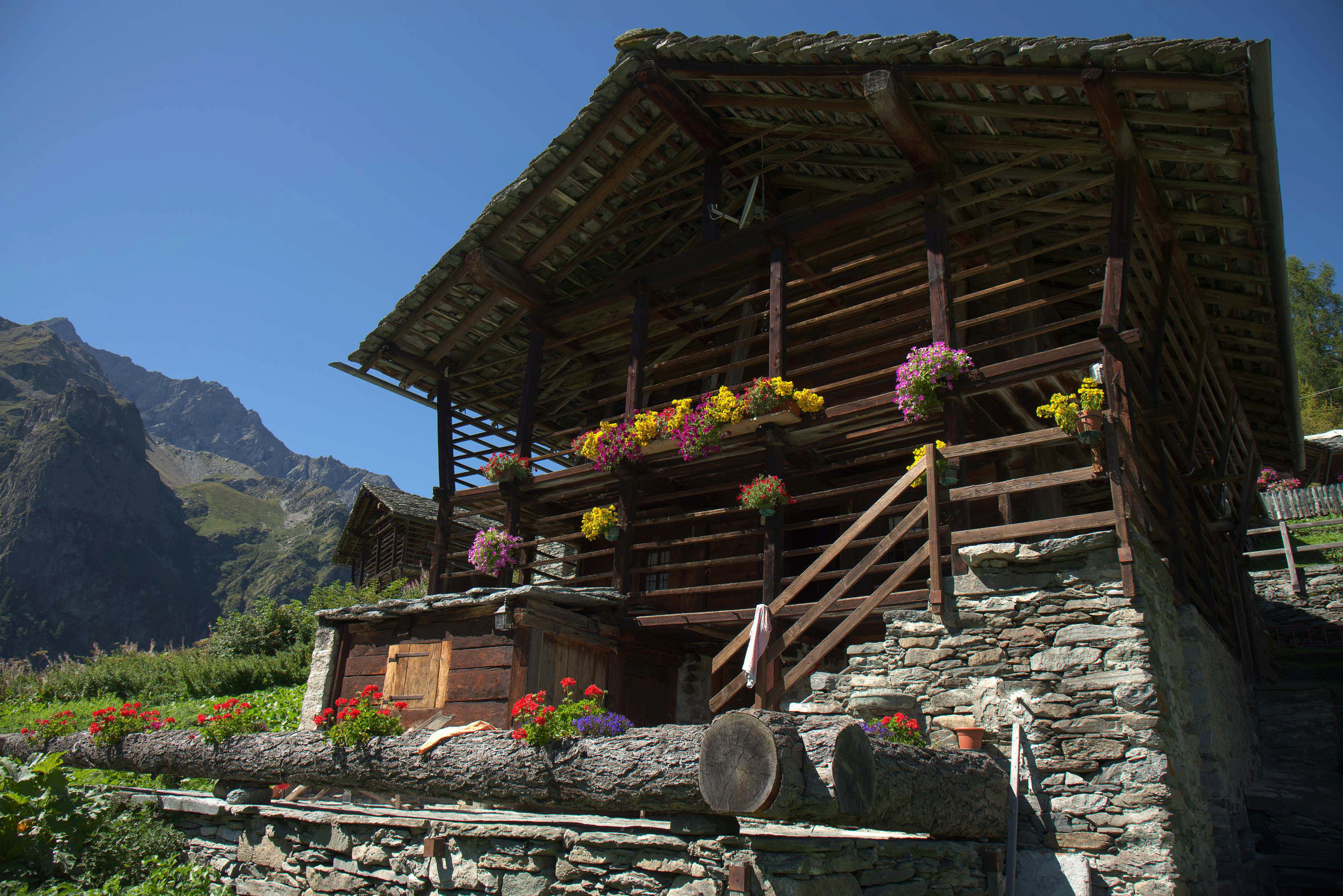
Other than for a couple of irrelevant objects, blown pixels relate mainly to specular reflection flecks in the stone, logs and flowers – but the subject of the image proper, including most of the flowers, fits pretty well within white-balanced raw bounds.   Since this is a wholly linear exercise I did not perform any highlight reconstruction but instead simply clipped every value to the same level as G’s maximum at this point,  per the procedure outlined in the article on rendering.

After multiplication of the white balanced and demosaiced raw data by the Forward Matrix the situation in XYZ is shown below.  We now have a few values being clipped (immaterial rounding errors, first frame of the animation below) and many being sent below zero (material, second frame):

The story here is all about the yellow flowers: there is a  little bit of clipping in the Y channel  (green in the animation) and a lot of negative Z values (blue in the animation).  There are also some negative values in the green foliage on the log.  The rest of the image, including the other flowers and the sky, pretty well all fit within XYZ space.

Clipping is a sign of ‘overexposure’, while negative values indicate raw data captured by the camera outside of the visible range, hence out-of-gamut ‘imaginary colors’.  Keep in mind that the images above show what colors are clipped but not by how much, so the end effect on the clipped color may or may not be substantial.

xy Chromaticities of the Capture

XYZ is considered a color space with direct correspondence to human perception of color.  In other words if two tones have the same coordinates in XYZ they should appear to have the same color to a human observer.  Therefore while in XYZ we can take a look at the data projected onto the classic Helmholtz chromaticity horseshoe, which is supposed to represent the limits of color vision^[4].

First I am going to show the chromaticity diagram of the white balanced ColorChecker target used to determine the color matrix of Figure 2, transformed into XYZ by the matrix we derived.

The 24 dots represent the chromaticities of the 24 patches.  The six gray patches in the bottom row of the ColorChecker are bunched up near the center of the horseshoe where D50 resides, as they should.  A couple of dots in the yellow-orange region appear to be just outside of sRGB (white solid line).  They actually could be – but recall from the previous article that the Forward Matrix is a compromise, with some noticeable errors.  Shown below are deviations from BabelColor 30 database reference data^[5].  One is supposed to represent a just noticeable difference.  Note that orange and yellow are indeed two of the worst offenders.

If every raw pixel of the image in Figure 1 is white balanced, demosaiced, converted to XYZ and plotted as in Figure 5 we get the chromaticities below left.  Too many dots, but it shows the gamut of chromaticities at the scene captured by a D610 and 24-120mm f/4 under the ‘daylight’ 5350K mountain sun.  Some values are indeed negative and some values fall outside of Helmholtz’ horseshoe, hence outside the limits of human vision.

Since it’s hard to determine from Figure 7a how many pixels correspond to each chromaticity,  the diagram on the right (7b)  shows instead a histogram of the number of pixels within the relative .01x.01 xy chromaticity square.  The counts are in log10 units and color coded, so dark blue means that there are less than 10  pixels in such a square, light blue less than 100, cyan less than 1000 … all the way to yellow with more than 100k.   We can then easily see where we are losing color information in what numbers by referencing the standard color gamuts (yellow, red and black triangles for sRGB, Adobe RGB and ProPhoto resp.).

For instance it would be a pity to lose chromaticities by the hundreds or thousands (indicated by cyan and green in the histograms of figures 7b and 8). Note that even Adobe RGB would not be quite enough for this scene and that the hardware is capturing colors that we cannot see (e.g. outside of the NW to SE going line of the ProPhoto color space, which coincides with the edge of the horseshoe).

It actually makes more sense to look at this data in the perceptually more uniform CIELUV color space:

The weighted histogram shows that image ‘colors’ fit better into the visible range.  The yellow dots, representing the most numerous chromaticities, obviously relate to the blue sky.

Taking It to sRGB

Now that we understand the limitations of the data in – and staying with our initial illumination assumption – we can multiply it by the standard matrix  that will take it to our chosen colorimetric ‘output’ color space, in this case , as discussed earlier.  I did not clip values below zero or above max in order to maintain linearity until the end. From Bruce Lindbloom’s site^[3]:

You can see that the coefficients in this matrix are much larger than those of the Forward Matrix shown in Figure 2, so they are much more aggressive on the data.  Indeed this is the step in the color rendering process that leaves the most information on the raw conversion floor, both clipping (first frame below, flowers etc.) and blocking (negative values, second frame, flowers and foliage).  Gray tones made it through to sRGB, colored items did not.

All those tones above full scale and below zero need to be clipped/blocked to fit into the sRGB color space and are therefore corrupted.   Interesting how much of the foliage did not make it through unscathed, though remember that Figure 9 just indicates that those colors are clipped, without showing how much they are outside of sRGB’s gamut.  Refer to figures 7 and 8 for that – and take a look at the article on just noticeable color differences on how to go about figuring out whether they would be noticeable.

WB Raw to sRGB in One Matrix

Alternatively in this case the full linear trip from white balanced and demosaiced raw data to sRGB could be accomplished by multiplying the two matrices above together, resulting in the following single matrix as discussed in the previous article

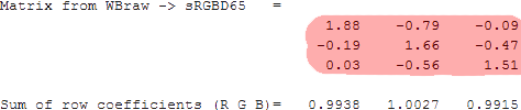
Ideally we would like the sum of the row coefficients to be all ones so that a neutral tone in the raw data (say [0.5 0.5 0.5]) would map to the same neutral tone in sRGB, but this is close enough considering the fact that a Forward Matrix is by definition a compromise.  If we forced the sums of all row coefficients to be equal to one, as most matrix generators do, then that would be accomplished at the expense of some other tones.   This being a landscape where whites are not critical I prefer to leave the matrix which yields the best overall color compromises as-is.

Also no point getting too finicky at this stage given the fact that we assumed illumination while in this case it turned out to be closer to .  The result is a slightly incorrect final image white balance, which however would be hardly noticeable under adapted conditions, as you can easily prove to yourself by playing with the WB slider of any raw coverter.

How Do You Like’m Linear Blues?

The final step in obtaining the image of Figure 1 is to apply sRGB gamma.  Here it is again below, followed by a few ‘flat’ renditions by real raw converters, after I tried to turn all corrections/curves off. All conversions were white balanced off the same gray ColorChecker patch but Figure 10 (the one we’ve been working on) was the only one that had the benefit of having the applied Forward Matrix designed from a ColorChecker Passport Photo under the correct illuminant at the time of capture.  If you click on one of them it opens up in a new tab where it can be zoomed to 1:1 if desired^[G].

Figure 10 and Figure 11 (mine and RawTherapee’s) are the purest linear renditions and look very similar, even though their Forward Matrices most likely are not.  I assume RT uses interpolated matrices from Adobe DNG.

I was not able to defeat all corrections in Capture NX-D and Adobe Camera Raw CC, hence the differences in color, contrast and chromaticity.  I know that ACR’s colors, and I am guessing CNX-D’s, are fine tuned non linearly during conversion.   In addition I believe they both apply a positive ‘Baseline Exposure’ correction, counting on nonlinear highlight correction algorithms in order not to clip then.  I had to apply -1.2 and -1.0 stops of EC to CNX-D and ACR respectively in order to keep their brightnesses roughly comparable to the other two.

Bonus: Nonlinear Blues

This article is about linear color, so no attempt was made to make the reference image more accurate through an ‘HSV map’ or more pleasing by applying ‘look’ and ‘tone curve’ fine tuning aimed at a specific class of output media like monitors.  The quoted terms refer to advanced color corrections applied in commercial raw converters.  Some of these corrections are applied while in XYZ space via round trips to ProPhotoRGB and HSV and back, per the DNG spec; others can just as well be applied via an editor like PhotoShop after rendering.

To give you an idea  of how the linearly converted image would look after such corrections, here is a version with a very mild custom profile generated by DcamProf with Anders Torger’s neutral+ operator^[6], as rendered by RawTherapee.  It is meant to be shown in Adobe RGB on a wide gamut monitor but I converted it to sRGB for wider consumption.  To see its real colors you should probably click on the image to open it in its own tab, save it and open it in a color managed editor like PhotoShop.

Beauty is in the eye of the beholder and lots of adjustments could be made in post to improve the image in Figure 10 for the intended display medium and purpose.  But in this case nothing at all was done to it other than white balance, demosaic by averaging the green channels in each quartet and apply color.  This concludes this short series on how (linear) color is rendered during raw conversion.

Gallery

The same five final images are assembled in a gallery below.  If you click on one of them they open up full screen and you can navigate between them using the superimposed left and right arrows.  The bottom left hand corner indicates the image you are viewing (sRGB is mine, the others are self explanatory).

Notes and References

<sub>1. Lots of provisos and simplifications for clarity as always.  I am not a color scientist, so if you spot any mistakes please let me know.
2. Minimally demosaiced means that for each quartet the Red and Blue values were taken as-is from the raw data, while Green was the average of the G1 and G2 raw values, equivalent to dcraw -h.
3. This is the link to Bruce Lindbloom’s site.
4. Helmholtz’s horseshoe was drawn by excellent matlab plugin optprop.
5. The ColorChecker pages at BabelColor.com can be found here. Careful that there was a change in formulations in November 2014.
6. Anders Torger’s site and his excellent profile maker DcamProf can be found here.</sub>