Ever since Einstein we’ve been able to say that humans ‘see’ because information about the scene is carried to the eyes by photons reflected by it. So when we talk about Information in photography we are referring to information about the energy and distribution of photons arriving from the scene. The more complete this information, the better we ‘see’. No photons = no information = no see; few photons = little information = see poorly = poor IQ; more photons = more information = see better = better IQ.
Sensors in digital cameras work similarly, their output ideally being the energy and location of every photon incident on them during Exposure. That’s the full information ideally required to recreate an exact image of the original scene for the human visual system, no more and no less. In practice however we lose some of this information along the way during sensing, so we need to settle for approximate location and energy – in the form of photoelectron counts by pixels of finite area, often correlated to a color filter array.
Let’s review a simple model of how this works. Photons strike the sensor and generate photoelectrons (e-) proportionally to available Luminance from the scene. The proportion is due to the physical characteristics of the equipment and camera setup: it is fixed for a given Exposure. The number and distribution of photoelectrons collected by the photosites in a sensor before any (including in-pixel) linear amplification represent the most complete description of information from the scene possible for the given setup and Exposure. We call this number and distribution the ‘Signal’, in units of e-. It is shown in red below (refer to the simple model article for additional details):

Defining The Signal and Noise
The Signal is not the number of e- collected by a single pixel because the level of a single pixel is not representative of incoming light intensity. Photons arrive in a well understood Poissonian distribution of time and space. And photoelectrons resulting from photons interacting with silicon are in turn generated according to Poisson statistics. So if we were to collect statistics on the e- count produced by a patch of pixels in a sensor after a set Exposure under uniform illumination we would find the distribution of the counts to be quite varied, with a well defined mean and standard deviation. On the other hand, thanks to quantum mechanics, the output of a single pixel could literally be anything from zero to full scale.
When talking about the Signal therefore we refer to the mean number of photoelectrons collected by a uniformly illuminated patch of pixels before any linear amplification, their standard deviation referred to as ‘Noise’. We call the number of pixels under examination the ‘sample size‘. Signal (s in the figure above) and Noise (n in the figure above) are very closely related and in some cases only one is needed to know the other. There can be no Signal without Noise. But there can be Noise without a signal.
Sources of Noise
There is always a certain amount of random noise present in a well designed imaging system, partly inherent in the Signal itself (Poissonian Shot Noise, √s above) and partly added by the electronics (Gaussian Read Noise, r in the figure above). This noise degrades the accuracy of measurement of the photoelectrons (e-) rolling off the sensor, influencing the accuracy of the imager and the precision required to fully record information collected by it.
There are many other sources of noise that limit the performance of a camera, but for this article we will limit ourselves to random ones including the above, non uniformities (p in the figure above) and quantization. Refer to these pages by Emil Martinec for a good introduction to digital camera noise.
As Good as it Gets: In-Sensor
The Signal and Noise immediately out of the photosites, before they are amplified and converted to raw values (DN in the figure), represent the most accurate and complete information from the scene (IQ) available to the design engineer and to the photographer, for the given camera setup and Exposure. It can only get worse from there. Any further manipulation of the Signal, including its amplification, storage, processing for rendering or PP has as its main objective the preservation of as much of this information as possible so that the final image will be based on the best IQ available.
Amazingly, the PTC Method allows us to estimate the inaccessible Signal within the pixels in its natural units of e- simply by analyzing the information contained in the raw data.
Information Straight off a Sensor
So let’s take a look at what the output of a sensor in units of e- may look like under uniform illumination assuming a Signal of 25e- and read noise of 5e-. Recall that for most current digital camera sensors this signal would be found in the deep shadows of a capture, the total random noise mostly a quadrature sum of shot noise (√25) and read noise (5). Theoretically then total noise would be 7.07e- ( =√50).
At these low Signal levels PRNU (s*p) can be ignored so this is what has been simulated below. For this example the region of interest is a small patch of arbitrarily chosen pixels inside the red circle:
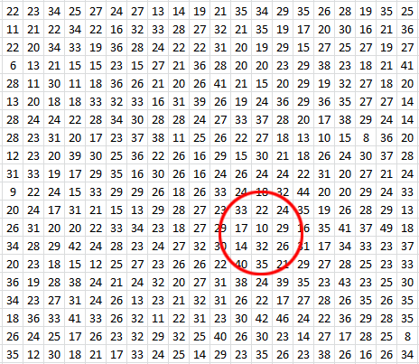
The 10 chosen values in our sample (33,22,24,17,10,29,14,32,26,35) show a mean signal of 24.20e- and a standard deviation ‘noise’ of 8.46e-.
SNR = mean / standard deviation
Since we now have a mean and a standard deviation from the sample we can calculate an IQ metric, their ratio – aptly called the Signal to Noise Ratio, which in this case is equal to 2.86. Quite low but still within the ‘engineering’ requirement that it be larger than 1 for an acceptable result.
We can compare these results to theoretical values for such a signal (25 e-), total noise (7.07e-) and their ratio: SNR (3.54). They are somewhat different from the ideal because the sample size is small and the individual pixel intensities are themselves quantized in integer units of e-: the information from the scene itself is not continuous (represented by Real, floating point numbers) but quantized (represented by Discrete, integer numbers). Thank you Planck.
If we move the circle around the uniformly lit area and each time calculate the above statistics we will find that the mean will oscillate around 25e- and the standard deviation around 7e-, but almost never exactly compute to the values that theory predicts because of spatial and temporal quantization. Don’t worry, our visual system is designed to work like this also, the red circle representing the eye’s Circle of Confusion on the retina.
Sample Size is Key
Assuming the sensor was uniformly illuminated, we could improve the accuracy of the measurement by enlarging the sample size, thus effectively averaging out the error introduced by quantization. This trick only works when there is enough noise in the system but not too much, as in this case.
For instance if the circle encompassed the entire 400 pixels shown, the mean signal would be 25.59e-, the standard deviation 7.41e- and SNR 3.45, closer to the values suggested by theory. As the sample size gets larger, precision improves:
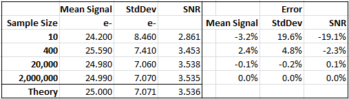
With a static scene we could also sample the area many separate times, increasing the number of available samples to compute Signal, Noise and SNR. Information theory suggests that to keep the sampling error below 1% one needs to have a sample size of 20,000 or more.
Next, how this information is amplified, converted by the ADC and stored in a raw file.