IQ, Optics, Sharpness, Spatial Resolution

What is Resolution?

May 8, 2024 Jack 5 Comments

In photography Resolution refers to the ability of an imaging system to capture fine detail from the scene, making it a key determinant of Image Quality. For instance, with high resolution equipment we might be able to count the number of tiny leaves on a distant tree, while we might not with a lower-res one. Or the leaves might look sharp with the former and unacceptably mushy with the latter.

We quantify resolution by measuring detail contrast after it has been inevitably smeared by the imaging process. As detail becomes smaller and closer together in the image, the blurred darker and lighter parts start mixing together until the relative contrast decreases to the point that it disappears, a limit referred to as diffraction extinction, beyond which all detail is lost and no additional spatial information can be captured from the scene.

Sinusoidal target of increasing frequency to diffraction limit extinction — Increasingly small detail smeared by the imaging process, highly magnified.

The units of resolution are spatial frequencies, the inverse of the size and distance of the detail in question. Of course at diffraction extinction no visual information is captured, therefore in most cases the criteria for usability are set by larger detail than that – or equivalently at lower frequencies. Thresholds tend to be application specific and arbitrary.

The type of resolution being measured must also be specified since the term can be applied to different physical quantities: sensor, spatial, temporal, spectral, type of light, medium etc. In photography we are normally interested in Spatial Resolution from incoherent light traveling in air so that will be the focus here.

Continue reading What is Resolution? →

Fourier Optics, MTF, PSF, Sharpness, Spatial Resolution

Introduction to Texture MTF

November 19, 2023 Jack 5 Comments

Texture MTF is a method to measure the sharpness of a digital camera and lens by capturing the image of a target of known characteristics. It purports to better evaluate the perception of fine details in low contrast areas of the image – what is referred to as ‘texture’ – in the presence of noise reduction, sharpening or other non-linear processing performed by the camera before writing data to file.

Figure 1. Image of Dead Leaves low contrast target. Such targets are designed to have controlled scale and direction invariant features with a power law Power Spectrum.

The Modulation Transfer Function (MTF) of an imaging system represents its spatial frequency response, from which many metrics related to perceived sharpness are derived: MTF50, SQF, SQRI, CMT Acutance etc. In these pages we have used to good effect the slanted edge method to obtain accurate estimates of a system’s MTF curves in the past.^[1]

In this article we will explore proposed methods to determine Texture MTF and/or estimate the Optical Transfer Function of the imaging system under test from a reference power-law Power Spectrum target. All three rely on variations of the ratio of captured to reference image in the frequency domain: straight Fourier Transforms; Power Spectral Density; and Cross Power Density. In so doing we will develop some intuitions about their strengths and weaknesses. Continue reading Introduction to Texture MTF →

illuminant, Information Science, Quantization, Sensors, SPD, variation

Photons, Shot Noise and Poisson Processes

May 17, 2023 Jack Leave a comment

Every digital photographer soon discovers that there are three main sources of visible random noise that affect pictures taken in normal conditions: Shot, pixel response non-uniformities (PRNU) and Read noise.^[1]

Shot noise (sometimes referred to as Photon Shot Noise or Photon Noise) we learn is ‘inherent in light’; PRNU is per pixel gain variation proportional to light, mainly affecting the brighter portions of our pictures; Read Noise is instead independent of light, introduced by the electronics and visible in the darker shadows. You can read in this earlier post a little more detail on how they interact.

However, shot noise is omnipresent and arguably the dominant source of visible noise in typical captures. This article’s objective is to dig deeper into the sources of Shot Noise that we see in our photographs: is it really ‘inherent in the incoming light’? What about if the incoming light went through clouds or was reflected by some object at the scene? And what happens to the character of the noise as light goes through the lens and is turned into photoelectrons by a pixel’s photodiode?

Fish, dear reader, fish and more fish.

Continue reading Photons, Shot Noise and Poisson Processes →

Fourier Optics, Geometrical Optics, MTF, PSF, wavefront

Fourier Optics and the Complex Pupil Function

April 13, 2023 Jack Leave a comment

In the last article we learned that a complex lens can be modeled as just an entrance pupil, an exit pupil and a geometrical optics black-box in between. Goodman^[1] suggests that all optical path errors for a given Gaussian point on the image plane can be thought of as being introduced by a custom phase plate at the pupil plane, delaying or advancing the light wavefront locally according to aberration function $\Delta W(u,v)$ as earlier described.

The phase plate distorts the forming wavefront, introducing diffraction and aberrations, while otherwise allowing us to treat the rest of the lens as if it followed geometrical optics rules. It can be associated with either the entrance or the exit pupil. Photographers are usually concerned with the effects of the lens on the image plane so we will associate it with the adjacent Exit Pupil.

aberrations coded as phase plate in exit pupil generalized complex pupil function — Figure 1. Aberrations can be fully described by distortions introduced by a fictitious phase plate inserted at the uv exit pupil plane. The phase error distribution is the same as the path length error described by wavefront aberration function ΔW(u,v), introduced in the previous article.

Continue reading Fourier Optics and the Complex Pupil Function →

Fourier Optics, Geometrical Optics, intensity, MTF, Optics, PSF, wavefront

An Introduction to Pupil Aberrations

March 17, 2023 Jack Leave a comment

As discussed in the previous article, so far we have assumed ideal optics, with spherical wavefronts propagating into and out of the lens’ Entrance and Exit pupils respectively. That would only be true if there were no aberrations. In that case the photon distribution within the pupils would be uniform and such an optical system would be said to be diffraction limited.

Figure 1. Optics as a black box, fully described for our purposes by its terminal properties at the Entrance and Exit pupils. A horrible attempt at perspective by your correspondent: the Object, Pupils and Image planes should all be parallel and share the optical axis z.

On the other hand if lens imperfections, aka aberrations, were present the photon distribution in the Exit Pupil would be distorted, thus unable to form a perfectly spherical wavefront out of it, with consequences for the intensity distribution of photons reaching the image.

Either pupil can be used to fully describe the light collection and concentration characteristics of a lens. In imaging we are typically interested in what happens after the lens so we will choose to associate the performance of the optics with the Exit Pupil. Continue reading An Introduction to Pupil Aberrations →

DOF, intensity, Optics, wavefront

Pupils and Apertures

March 15, 2023 Jack 4 Comments

We’ve seen in the last article that the job of an ideal photographic lens is simple: to receive photons from a set of directions bounded by a spherical cone with its apex at a point on the object; and to concentrate them in directions bounded by a spherical cone with its apex at the corresponding point on the image. In photography both cones are assumed to be in air.

In this article we will distill the photon collecting and distributing function of a complex lens down to its terminal properties, the Entrance and Exit Pupils, allowing us to deal with any lens simply and consistently. Continue reading Pupils and Apertures →

Exposure, imaging system, irradiance, luminance, radiance, Radiometry, reflectance, Uncategorized

Angles and the Camera Equation

February 26, 2023 Jack Leave a comment

Imagine a bucolic scene on a clear sunny day at the equator, sand warmed by the tropical sun with a typical irradiance ( $E$ ) of about 1000 watts per square meter. As discussed earlier we could express this quantity as illuminance in lumens per square meter ( $lx$ ) – or as a certain number of photons per second ( $\Phi$ ) over an area of interest ( $\mathcal{A}$ ).

(1) $\begin{equation*} E = \frac{\Phi}{\mathcal{A}} \; (W, lm, photons/s) / m^2 \end{equation*}$

How many $photons/s$ per unit area can we expect on the camera’s image plane (irradiance $E_i$ )?

Figure 1. Irradiation transfer from scene to sensor.

In answering this question we will discover the Camera Equation as a function of opening angles – and set the stage for the next article on lens pupils. By the way, all quantities in this article depend on wavelength and position in the Field of View, which will be assumed in the formulas to make them readable, see Appendix I for a more formally correct version of Equation (1).

Continue reading Angles and the Camera Equation →

ACR, cct, Color, DNG, white balance, white point

Off Balance

May 16, 2022 Jack Leave a comment

In this article we confirm quantitatively that getting the White Point, hence the White Balance, right is essential to obtaining natural tones out of our captures. How quickly do colors degrade if the estimated Correlated Color Temperature is off?

Continue reading Off Balance →

adobe camera raw, Color

A Question of Balance

May 9, 2022 Jack Leave a comment

In this article I bring together qualitatively the main concepts discussed in the series and argue that in many (most) cases a photographer’s job in order to obtain natural looking tones in their work during raw conversion is to get the illuminant and relative white balance right – and to step away from any slider found in menus with the word ‘color’ in them.

Figure 1. DON’T touch them color dials (including Tint)! courtesy of Capture One

If you are an outdoor photographer trying to get balanced greens under an overcast sky – or a portrait photographer after good skin tones – dialing in the appropriate scene, illuminant and white balance puts the camera/converter manufacturer’s color science to work and gets you most of the way there safely. Of course the judicious photographer always knew to do that – hopefully now with a better appreciation as for why.

Continue reading A Question of Balance →

Color, color science, correlated color temperature

White Point, CCT and Tint

May 9, 2022 Jack 2 Comments

As we have seen in the previous post, knowing the characteristics of light at the scene is critical to be able to determine the color transform that will allow captured raw data to be naturally displayed from an output color space like ubiquitous sRGB.

White Point

The light source Spectral Power Distribution (SPD) corresponds to a unique White Point, namely a set of coordinates in the $XYZ$ color space, obtained by multiplying wavelength-by-wavelength its SPD (the blue curve below) by the response of the retina of a typical viewer, otherwise known as the CIE Color Matching Functions of a Standard Observer ( $\hat{x},\hat{y},\hat{z}$ in the plot)

Figure 1. Spectral Power Distribution of Standard Daylight Illuminant D5300 with a Correlated Color Temperature of 5300 deg. K; and CIE (2012) 2-deg XYZ “physiologically relevant” Color Matching Functions from cvrl.org.

Adding (integrating) the three resulting curves we get three values that represent the illuminant’s coordinates in the $XYZ$ color space. The White Point is obtained by dividing these coordinates by the $Y$ value to normalize it to 1.

For example a Standard Daylight Illuminant with a Correlated Color Temperature of 5300 kelvins has a White Point of^[1]

$XYZn$ = [0.9593 1.0000 0.8833]

assuming CIE (2012) 2-deg XYZ “physiologically relevant” Color Matching Functions from cvrl.org. Continue reading White Point, CCT and Tint →

Color, DNG, xyz

Linear Color Transforms

April 30, 2022 Jack 6 Comments

Building on a preceeding article of this series, once demosaiced raw data from a Bayer Color Filter Array sensor represents the captured image as a set of triplets, corresponding to the estimated light intensity at a given pixel under each of the three spectral filters part of the CFA. The filters are band-pass and named for the representative peak wavelength that they let through, typically red, green, blue or $r$ , $g$ , $b$ for short.

Since the resulting intensities are linearly independent they can form the basis of a 3D coordinate system, with each $rgb$ triplet representing a point within it. The system is bounded in the raw data by the extent of the Analog to Digital Converter, with all three channels spanning the same range, from Black Level with no light to clipping with maximum recordable light. Therefore it can be thought to represent a space in the form of a cube – or better, a parallelepiped – with the origin at [0,0,0] and the opposite vertex at the clipping value in Data Numbers, expressed as [1,1,1] if we normalize all data by it.

Figure 1. The linear sRGB Cube, courtesy of Matlab toolbox Optprop.

The job of the color transform is to project demosaiced raw data $rgb$ to a standard output $RGB$ color space designed for viewing. Such spaces have names like $sRGB$ , $Adobe RGB$ or $Rec. 2020$ . The output space can also be shown in 3D as a parallelepiped with the origin at [0,0,0] with no light and the opposite vertex at [1,1,1] with maximum displayable light. Continue reading Linear Color Transforms →

Color, Perceptual, Sharpness

Cone Fundamentals & the LMS Color Space

December 13, 2021 Jack 2 Comments

In the last article we showed how a digital camera’s captured raw data is related to Color Science. In my next trick I will show that CIE 2012 2 deg XYZ Color Matching Functions $\bar{x}$ , $\bar{y}$ , $\bar{z}$ displayed in Figure 1 are an exact linear transform of Stockman & Sharpe (2000) 2 deg Cone Fundamentals $\bar{\rho}$ , $\bar{\gamma}$ , $\bar{\beta}$ displayed in Figure 2

(1) $\begin{equation*} \left[ \begin{array}{c} \bar{x}} \\ \bar{y} \\ \bar{z} \end{array} \right] = M_{lx} * \left[ \begin{array} {c}\bar{\rho} \\ \bar{\gamma} \\ \bar{\beta} \end{array} \right] \end{equation*}$

with CMFs and CFs in 3xN format, $M_{lx}$ a 3×3 matrix and $*$ matrix multiplication. Et voilà:^[1]

Figure 1. Solid lines: CIE (2012) 2° XYZ “physiologically-relevant” Colour Matching Functions and photopic Luminous Efficiency Function (V) from cvrl.org, the Colour & Vision Research Laboratory at UCL. Dotted lines: The Cone Fundamentals in Figure 2 after linear transformation by 3×3 matrix Mlx below. Source: cvrl.org.

Continue reading Cone Fundamentals & the LMS Color Space →

Color, Exposure, Photometry, Radiometry, Sensors

Connecting Photographic Raw Data to Tristimulus Color Science

December 9, 2021 Jack Leave a comment

Absolute Raw Data

In the previous article we determined that the three $r_{_L}g_{_L}b_{_L}$ values recorded in the raw data in the center of the image plane in units of Data Numbers per pixel – by a digital camera and lens as a function of absolute spectral radiance $L(\lambda)$ at the lens – can be estimated as follows:

(1) $\begin{equation*} r_{_L}g_{_L}b_{_L} =\frac{\pi p^2 t}{4N^2} \int\limits_{380}^{780}L(\lambda) \odot SSF_{rgb}(\lambda) d\lambda \end{equation*}$

with subscript $_L$ indicating absolute-referred units and $SSF_{rgb}$ the three system Spectral Sensitivity Functions. In this series of articles $\odot$ is wavelength by wavelength multiplication (what happens to the spectrum of light as it progresses through the imaging system) and the integral just means the area under each of the three resulting curves (integration is what the pixels do during exposure). Together they represent an inner or dot product. All variables in front of the integral were previously described and can be considered constant for a given photographic setup. Continue reading Connecting Photographic Raw Data to Tristimulus Color Science →

Color, Exposure, Photometry, Radiometry, Sensors

The Physical Units of Raw Data

November 13, 2021 Jack Leave a comment

In the previous article we (I) learned that the Spectral Sensitivity Functions of a given digital camera and lens are the result of the interaction of light from the scene with all of the spectrally varied components that make up the imaging system: mainly the lens, ultraviolet/infrared hot mirror, Color Filter Array and other filters, finally the photoelectric layer of the sensor, which is normally silicon in consumer kit.

Figure 1. The journey of light from source to sensor. Cone Ω will play a starring role in the narrative that follows.

In this one we will put the process on a more formal theoretical footing, setting the stage for the next few on the role of white balance.

Continue reading The Physical Units of Raw Data →

Color, Exposure, Photometry, Radiometry, Sensors

The Spectral Response of Digital Cameras

November 10, 2021 Jack 2 Comments

Photography works because visible light from one or more sources reaches the scene and is reflected in the direction of the camera, which then captures a signal proportional to it. The journey of light can be described in integrated units of power all the way to the sensor, for instance so many watts per square meter. However ever since Newton we have known that such total power is in fact the result of the weighted sum of contributions by every frequency that makes up the light, what he called its spectrum.

Our ability to see and record color depends on knowing the distribution of the power contained within a subset of these frequencies and how it interacts with the various objects in its path. This article is about how a typical digital camera for photographers interacts with the spectrum arriving from the scene: we will dissect what is sometimes referred to as the system’s Spectral Response or Sensitivity.

Figure 1. Spectral Sensitivity Functions of an arbitrary imaging system, resulting from combining the responses of the various components described in the article.

Continue reading The Spectral Response of Digital Cameras →

IQ, Raspberry Pi, Sensors

Pi HQ Cam Sensor Performance

May 17, 2020 Jack 13 Comments

Now that we know how to open 12-bit raw files captured with the new Raspberry Pi High Quality Camera, we can learn a bit more about the capabilities of its 1/2.3″ Sony IMX477 sensor from a keen photographer’s perspective. The subject is a bit dry, so I will give you the summary upfront. These figures were obtained with my HQ module at room temperature and the raspistill – -raw (-r) command:

Raspberry Pi HQ Camera	raspistill --raw -ag 1	Comments
Black Level	256.3 DN	256.0 - 257.3 based on gain
White Level	4095	Constant throughout
Analog Gain	1	Gain Range 1 - 16
Read Noise	3 e-, gain 1 1.5 e-, gain 16	1.53 DN from black frame 11.50 DN
Clipping (FWC)	8180 e-	at base gain, 3400e-/um^2
Dynamic Range	11.15 stops 11.3 stops	SNR = 1 to Clipping Read Noise to Clipping
System Gain	0.47 DN/e-	at base analog gain
Star Eater Algorithm	Partly Defeatable	All channels - from base gain and from min shutter speed
Low Pass Filter	Yes	All channels - from base gain and from min shutter speed

Continue reading Pi HQ Cam Sensor Performance →

Color, Formats, Processing, Raspberry Pi, Sensors

Opening Raspberry Pi High Quality Camera Raw Files

May 15, 2020 Jack 17 Comments

The Raspberry Pi Foundation recently released an interchangeable lens camera module based on the Sony IMX477, a 1/2.3″ back side illuminated sensor with 3040×4056 pixels of 1.55um pitch. In this somewhat technical article we will unpack the 12-bit raw still data that it produces and render it in a convenient color space.

still life raw capture data file raspberry pi high quality hq cam f/8 1/2s base analog gain iso adobe rgb — Figure 1. 12-bit raw capture by Raspberry Pi High Quality Camera with 16 mm kit lens at f/8, 1/2 s, base ISO. The image was loaded into Matlab and rendered Half Height Nearest Neighbor in the Adobe RGB color space with a touch of local contrast and sharpening. Click on it to see it in its own tab and view it at 100% magnification. If your browser is not color managed you may not see colors properly.

Continue reading Opening Raspberry Pi High Quality Camera Raw Files →

DOF, Optics, Sensors, Sharpening, Sharpness, Spatial Resolution

Diffracted DOF Aperture Guides: 24-35mm

April 9, 2020 Jack 12 Comments

As a landscape shooter I often wonder whether old rules for DOF still apply to current small pixels and sharp lenses. I therefore roughly measured the spatial resolution performance of my Z7 with 24-70mm/4 S in the center to see whether ‘f/8 and be there’ still made sense today. The journey and the diffraction-simple-aberration aware model were described in the last few posts. The results are summarized in the Landscape Aperture-Distance charts presented here for the 24, 28 and 35mm focal lengths.

I also present the data in the form of a simplified plot to aid making the right compromises when the focusing distance is flexible. This information is valid for the Z7 and kit in the center only. It probably just as easily applies to cameras with similarly spec’d pixels and lenses. Continue reading Diffracted DOF Aperture Guides: 24-35mm →

DOF, IQ, Perceptual, Sharpness, Spatial Resolution

DOF and Diffraction: 24mm Guidelines

March 29, 2020 Jack 2 Comments

After an exhausting two and a half hour hike you are finally resting, sitting on a rock at the foot of your destination, a tiny alpine lake, breathing in the thin air and absorbing the majestic scenery. A cool light breeze suddenly rips the surface of the water, morphing what has until now been a perfect reflection into an impressionistic interpretation of the impervious mountains in the distance.

The beautiful flowers in the foreground are so close you can touch them, the reflection in the water 10-20m away, the imposing mountains in the background a few hundred meters further out. You realize you are hungry. As you search the backpack for the two panini you prepared this morning you begin to ponder how best to capture the scene: subject, composition, Exposure, Depth of Field.

Figure 1. A typical landscape situation: a foreground a few meters away, a mid-ground a few tens and a background a few hundred meters further out. Three orders of magnitude. The focus point was on the running dog, f/16, 1/100s. Was this a good choice?

Depth of Field. Where to focus and at what f/stop? You tip your hat and just as you look up at the bluest of blue skies the number 16 starts enveloping your mind, like rays from the warm noon sun. You dial it in and as you squeeze the trigger that familiar nagging question bubbles up, as it always does in such conditions. If this were a one shot deal, was that really the best choice?

In this article we attempt to provide information to make explicit some of the trade-offs necessary in the choice of Aperture for 24mm landscapes. The result of the process is a set of guidelines. The answers are based on the previously introduced diffraction-aware model for sharpness in the center along the depth of the field – and a tripod-mounted Nikon Z7 + Nikkor 24-70mm/4 S kit lens at 24mm.
Continue reading DOF and Diffraction: 24mm Guidelines →

IQ, Optics, Perceptual, Sharpness, Spatial Resolution

DOF and Diffraction: Setup

March 17, 2020 Jack 1 Comment

The two-thin-lens model for precision Depth Of Field estimates described in the last two articles is almost ready to be deployed. In this one we will describe the setup that will be used to develop the scenarios that will be outlined in the next one.

The beauty of the hybrid geometrical-Fourier optics approach is that, with an estimate of the field produced at the exit pupil by an on-axis point source, we can generate the image of the resulting Point Spread Function and related Modulation Transfer Function.

Pretend that you are a photon from such a source in front of a f/2.8 lens focused at 10m with about 0.60 microns of third order spherical aberration – and you are about to smash yourself onto the ‘best focus’ observation plane of your camera. Depending on whether you leave exactly from the in-focus distance of 10 meters or slightly before/after that, the impression you would leave on the sensing plane would look as follows:

Figure 1. PSF of a lens with about 0.6um of third order spherical aberration focused on 10m.

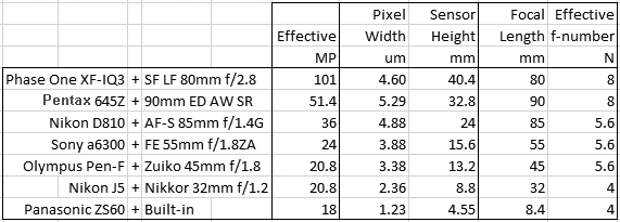
The width of the square above is 30 microns (um), which corresponds to the diameter of the Circle of Confusion used for old-fashioned geometrical DOF calculations with full frame cameras. The first ring of the in-focus PSF at 10.0m has a diameter of about 2.44 $\lambda \frac{f}{D}$ = 3.65 microns. That’s about the size of the estimated effective square pixel aperture of the Nikon Z7 camera that we are using in these tests.
Continue reading DOF and Diffraction: Setup →

Optics, Perceptual, Sharpness, Spatial Resolution

DOF and Diffraction: Image Side

March 11, 2020 Jack Leave a comment

This investigation of the effect of diffraction on Depth of Field is based on a two-thin-lens model, as suggested by Alan Robinson^[1]. We chose this model because it allows us to associate geometrical optics with one lens and Fourier optics with the other, thus simplifying the underlying math and our understanding.

In the last article we discussed how the front element of the model could present at the rear element the wavefront resulting from an on-axis source as a function of distance from the lens. We accomplished this by using simple geometry in complex notation. In this one we will take the relative wavefront present at the exit pupil and project it onto the sensing plane, taking diffraction into account numerically. We already know how to do it since we dealt with this subject in the recent past.

Figure 1. Where is the plane with the Circle of Least Confusion? Through Focus Line Spread Function Image of a lens at f/2.8 with the indicated third order spherical aberration coefficient, and relative measures of ‘sharpness’ MTF50 and Acutance curves. Acutance is scaled to the same peak as MTF50 for ease of comparison and refers to my typical pixel peeping conditions: 100% zoom, 16″ away from my 24″ monitor.

Continue reading DOF and Diffraction: Image Side →

Optics, Perceptual, Sharpness

DOF and Diffraction: Object Side

March 10, 2020 Jack 1 Comment

In this and the following articles we shall explore the effects of diffraction on Depth of Field through a two-lens model that separates geometrical and Fourier optics in a way that keeps the math simple, though via complex notation. In the process we will gain a better understanding of how lenses work.

The results of the model are consistent with what can be obtained via classic DOF calculators online but should be more precise in critical situations, like macro photography. I am not a macro photographer so I would be interested in validation of the results of the explained method by someone who is.

Figure 1. Simple two-thin-lens model for DOF calculations in complex notation. Adapted under licence.

Continue reading DOF and Diffraction: Object Side →

IQ, Optics, Sharpness, Spatial Resolution

The Nikon Z7’s Insane Sharpness

January 27, 2020 Jack 13 Comments

Ever since getting a Nikon Z7 MILC a few months ago I have been literally blown away by the level of sharpness it produces. I thought that my surprise might be the result of moving up from 24 to 45.7MP, or the excellent pin-point focusing mode, or the lack of an Antialiasing filter. Well, it turns out that there is probably more at work than that.

This weekend I pulled out the largest cutter blade I could find and set it up rough and tumble near vertically about 10 meters away to take a peek at what the MTF curves that produce such sharp results might look like.

Continue reading The Nikon Z7’s Insane Sharpness →

IQ, Sensors, Sharpness, Spatial Resolution

Canon’s High-Res Optical Low Pass Filter

January 15, 2020 Jack 7 Comments

Canon recently introduced its EOS-1D X Mark III Digital Single-Lens Reflex [Edit: and now also possibly the R5 Mirrorless ILC] touting a new and improved Anti-Aliasing filter, which they call a High-Res Gaussian Distribution LPF, claiming that

“This not only helps to suppress moiré and color distortion,
but also improves resolution.”

Figure 1. Artist’s rendition of new High-res Low Pass Filter, courtesy of Canon USA

In this article we will try to dissect the marketing speak and understand a bit better the theoretical implications of the new AA. For the abridged version, jump to the Conclusions at the bottom. In a picture:

Canon High-Res Anti-Aliasing filter — Figure 16: The less psychedelic, the better.

Continue reading Canon’s High-Res Optical Low Pass Filter →

Banding, IQ, Sensors

The HV Spectrogram

November 16, 2019 Jack 3 Comments

A spectrogram, also sometimes referred to as a periodogram, is a visual representation of the Power Spectrum of a signal. Power Spectrum answers the question “How much power is contained in the frequency components of the signal”. In digital photography a Power Spectrum can show the relative strength of repeating patterns in captures and whether processing has been applied.

In this article I will describe how you can construct a spectrogram and how to interpret it, using dark field raw images taken with the lens cap on as an example. This can tell us much about the performance of our imaging devices in the darkest shadows and how well tuned their sensors are there.

Pixel level noise spectrum — Figure 1. Horizontal and Vertical Spectrogram of noise captured in the raw data by a Nikon Z7 at base ISO with the lens cap on. The plot shows clear evidence of low-pass filtering in the blue CFA color plane and pattern noise repeating every 6 rows there and in one of the green ones.

Continue reading The HV Spectrogram →

Deconvolution, Sharpening, unsharp mask, USM

The Richardson-Lucy Algorithm

May 23, 2019 Jack 12 Comments

Deconvolution by the Richardson-Lucy algorithm is achieved by minimizing the convex loss function derived in the last article

(1) $\begin{equation*} J(O) = \sum \bigg (O**PSF - I\cdot ln(O**PSF) \bigg) \end{equation*}$

with

$J$ , the scalar quantity to minimize, function of ideal image $O(x,y)$
$I(x,y)$ , linear captured image intensity laid out in $M$ rows and $N$ columns, corrupted by Poisson noise and blurred by the $PSF$
$PSF(x,y)$ , the known two-dimensional Point Spread Function that should be deconvolved out of $I$
$O(x,y)$ , the output image resulting from deconvolution, ideally without shot noise and blurring introduced by the $PSF$
** two-dimensional convolution
$\cdot$ element-wise product
$ln$ , element-wise natural logarithm

In what follows indices $x$ and $y$ , from zero to $M$ -1 and $N$ -1 respectively, are dropped for readability. Articles about algorithms are by definition dry so continue at your own peril.

So, given captured raw image $I$ blurred by known function $PSF$ , how do we find the minimum value of $J$ yielding the deconvolved image $O$ that we are after?

Continue reading The Richardson-Lucy Algorithm →

Deconvolution, Processing, Sharpening

Elements of Richardson-Lucy Deconvolution

May 3, 2019 Jack 3 Comments

We have seen that deconvolution by naive division in the frequency domain only works in ideal conditions not typically found in normal photographic settings, in part because of shot noise inherent in light from the scene. Half a century ago William Richardson (1972)^[1] and Leon Lucy (1974)^[2] independently came up with a better way to deconvolve blurring introduced by an imaging system in the presence of shot noise. Continue reading Elements of Richardson-Lucy Deconvolution →

Deconvolution, Sharpening

Deconvolution by Naive Division

April 12, 2019 Jack Leave a comment

Now that we have the lens Point Spread Function it should be straight forward to reverse its blurring effect out of the image, right?

Figure 1. Lens PSF

Continue reading Deconvolution by Naive Division →

Deconvolution, IQ, Optics, Sharpening, Sharpness, Spatial Resolution

Capture Sharpening: Estimating Lens PSF

February 26, 2019 Jack Leave a comment

The next few articles will outline the first tiny few steps towards achieving perfect capture sharpening, that is deconvolution of an image by the Point Spread Function (PSF) of the lens used to capture it. This is admittedly a complex subject, fraught with a myriad ever changing variables even in a lab, let alone in the field. But studying it can give a glimpse of the possibilities and insights into the processes involved.

I will explain the steps I followed and show the resulting images and measurements. Jumping the gun, the blue line below represents the starting system Spatial Frequency Response (SFR)^[1], the black one unattainable/undesirable perfection and the orange one the result of part of the process outlined in this series.

Figure 1. Spatial Frequency Response of the imaging system before and after Richardson-Lucy deconvolution by the PSF of the lens that captured the original image.

Continue reading Capture Sharpening: Estimating Lens PSF →

Color

Phone Camera Color ‘Accuracy’

April 19, 2018 Jack 2 Comments

Just in case anyone was wondering (I was), it turns out that my smartphone camera produces a better SMI color score off a ColorChecker Passport target than a full frame Nikon D610 DSLR .

My latest phone, a late 2017 incarnation of the LG V34, produces raw DNG files, so I went poking around. From what I could gather the sensor is most likely Sony’s IMX 234^[1], 1/2.6″, Back Side Illuminated, stacked and based on the latest and cleanest Exmor RS technology. The sensor’s 1.12um pixels produce 16MP raw files with 10-bit depth, which I understand to be typical for current phone cameras. Other features include phase detect AF, an electronic shutter with variable integration time, HDR, hot pixel suppression and raw noise reduction (ugh!) – plus a slew of video features. Continue reading Phone Camera Color ‘Accuracy’ →

Color

A Just Noticeable Color Difference

January 25, 2018 Jack 9 Comments

While checking some out-of-gamut tones on an xy Chromaticity Diagram I started to wonder how far two tones needed to be in order for an observer to notice a difference. Were the tones in the yellow and red clusters below discernible or would they be indistinguishable, all being perceived as the same ‘color’?

Figure 1. Samples off an image plotted on a typical xy Chromaticity diagram (black dots).

Continue reading A Just Noticeable Color Difference →

Color, IQ

The Perfect Color Filter Array

January 20, 2018 Jack 14 Comments

We’ve seen how humans perceive color in daylight as a result of three types of photoreceptors in the retina called cones that absorb wavelengths of light from the scene with different sensitivities to the arriving spectrum.

A photographic digital imager attempts to mimic the workings of cones in the retina by usually having different color filters arranged in an array (CFA) on top of its photoreceptors, which we normally call pixels. In a Bayer CFA configuration there are three filters named for the predominant wavelengths that each lets through (red, green and blue) arranged in quartets such as shown below:

Figure 2. Bayer Color Filter Array: RGGB layout. Image under license from Cburnett, pixels shifted and text added.

A CFA is just one way to copy the action of cones: Foveon for instance lets the sensing material itself perform the spectral separation. It is the quality of the combined spectral filtering part of the imaging system (lenses, UV/IR, CFA, sensing material etc.) that determines how accurately a digital camera is able to capture color information from the scene. So what are the characteristics of better systems and can perfection be achieved? In this article I will pick up the discussion where it was last left off and, ignoring noise for now, attempt to answer this question using CIE conventions, in the process gaining insight in the role of the compromise color matrix and developing a method to visualize its effects.^[1] Continue reading The Perfect Color Filter Array →

Color, IQ, Processing, Sensors

Phase One IQ3 100MP Trichromatic vs Standard Back Linear Color, Part III

January 11, 2018 Jack Leave a comment

Over the last two posts we’ve been exploring some of the differences introduced by tweaks to the Color Filter Array of the Phase One IQ3 100MP Trichromatic Digital Back versus its original incarnation, the Standard Back. Refer to those for the background. In this article we will delve into some of these differences quantitatively^[1].

Let’s start with the compromise color matrices we derived from David Chew’s captures of a ColorChecher 24 in the shade of a sunny November morning in Ohio^[2]. These are the matrices necessary to convert white balanced raw data to the perceptual CIE XYZ color space, where it is said there should be one-to-one correspondence with colors as perceived by humans, and therefore where most measurements are performed. They are optimized for each back in the current conditions but they are not perfect, the reason for the word ‘compromise’ in their name:

Figure 1. Optimized Linear Compromise Color Matrices for the Phase One IQ3 100 MP Standard and Trichromatic Backs under approximately D65 light.

Continue reading Phase One IQ3 100MP Trichromatic vs Standard Back Linear Color, Part III →

Color, Processing, Sensors

Phase One IQ3 100MP Trichromatic vs Standard Back Linear Color, Part II

January 10, 2018 Jack Leave a comment

We have seen in the last post that Phase One apparently performed a couple of main tweaks to the Color Filter Array of its Medium Format IQ3 100MP back when it introduced the Trichromatic: it made the shapes of color filter sensitivities more symmetric by eliminating residual transmittance away from the peaks; and it boosted the peak sensitivity of the red (and possibly blue) filter. It did this with the objective of obtaining more accurate, less noisy color out of the hardware, requiring less processing and weaker purple fringing to boot.

Both changes carry the compromises discussed in the last article so the purpose of this one and the one that follows is to attempt to measure – within the limits of my tests, procedures and understanding^[1] – the effect of the CFA changes from similar raw captures by the IQ3 100MP Standard Back and Trichromatic, courtesy of David Chew. We will concentrate on color accuracy, leaving purple fringing for another time.

Figure 1. Phase One IQ3 100MP image rendered linearly via a dedicated color matrix from raw data without any additional processing whatsoever: no color corrections, no tone curve, no sharpening, no nothing. Brightness adjusted to just avoid clipping. Capture by David Chew.

Continue reading Phase One IQ3 100MP Trichromatic vs Standard Back Linear Color, Part II →

Color, Formats, IQ, Sensors

Phase One IQ3 100MP Trichromatic vs Standard Back Linear Color, Part I

January 8, 2018 Jack 2 Comments

It is always interesting when innovative companies push the envelope of the state-of-the-art of a single component in their systems because a lot can be learned from before and after comparisons. I was therefore excited when Phase One introduced a Trichromatic version of their Medium Format IQ3 100MP Digital Back last September because it could allows us to isolate the effects of tweaks to their Bayer Color Filter Array, assuming all else stays the same.

Figure 1. IQ3 100MP Trichromatic (left) vs the rest (right), from PhaseOne.com. Units are not specified but one would assume that the vertical axis is relative spectral sensitivity and the horizontal axis represents wavelength.

Thanks to two virtually identical captures by David Chew at getDPI, and Erik Kaffehr’s intelligent questions at DPR, in the following articles I will explore the effect on linear color of the new Trichromatic CFA (TC) vs the old one on the Standard Back (SB). In the process we will discover that – within the limits of my tests, procedures and understanding^[1] – the Standard Back produces apparently more ‘accurate’ color while the Trichromatic produces better looking matrices, potentially resulting in ‘purer’ signals. Continue reading Phase One IQ3 100MP Trichromatic vs Standard Back Linear Color, Part I →

Color, IQ, Sharpness, Spatial Resolution

Bayer CFA Effect on Sharpness

September 10, 2017 Jack Leave a comment

In this article we shall find that the effect of a Bayer CFA on the spatial frequencies and hence the ‘sharpness’ information captured by a sensor compared to those from the corresponding monochrome version can go from (almost) nothing to halving the potentially unaliased range – based on the chrominance content of the image and the direction in which the spatial frequencies are being stressed. Continue reading Bayer CFA Effect on Sharpness →

Optics, Quantization, Sensors, Spatial Resolution

Wavefront to PSF to MTF: Physical Units

February 19, 2017 Jack 2 Comments

In the last article we saw that the intensity Point Spread Function and the Modulation Transfer Function of a lens could be easily approximated numerically by applying Discrete Fourier Transforms to its generalized exit pupil function $\mathcal{P}$ twice in sequence.^[1]

Obtaining the 2D DFTs is easy: simply feed MxN numbers representing the two dimensional complex image of the Exit Pupil function in its $uv$ space to a Fast Fourier Transform routine and, presto, it produces MxN numbers representing the amplitude of the PSF on the $xy$ sensing plane. Figure 1a shows a simple case where pupil function $\mathcal{P}$ is a uniform disk representing the circular aperture of a perfect lens with MxN = 1024×1024. Figure 1b is the resulting intensity PSF.

Figure 1a, left: A circular array of ones appearing as a white disk on a black background, representing a circular aperture. Figure 1b, right: Array of numbers representing the PSF of image 1a in the classic shape of an Airy Pattern. — Figure 1. 1a Left: Array of numbers representing a circular aperture (zeros for black and ones for white). 1b Right: Array of numbers representing the PSF of image 1a (contrast slightly boosted).

Simple and fast. Wonderful. Below is a slice through the center, the 513th row, zoomed in. Hmm…. What are the physical units on the axes of displayed data produced by the DFT? Continue reading Wavefront to PSF to MTF: Physical Units →

Optics, Photometry, Quantization, Radiometry, Sensors, Spatial Resolution

Aberrated Wave to Image Intensity to MTF

February 18, 2017 Jack Leave a comment

Goodman, in his excellent Introduction to Fourier Optics^[1], describes how an image is formed on a camera sensing plane starting from first principles, that is electromagnetic propagation according to Maxwell’s wave equation. If you want the play by play account I highly recommend his math intensive book. But for the budding photographer it is sufficient to know what happens at the Exit Pupil of the lens because after that the transformations to Point Spread and Modulation Transfer Functions are straightforward, as we will show in this article.

The following diagram exemplifies the last few millimeters of the journey that light from the scene has to travel in order to be absorbed by a camera’s sensing medium. Light from the scene in the form of field $U$ arrives at the front of the lens. It goes through the lens being partly blocked and distorted by it as it arrives at its virtual back end, the Exit Pupil, we’ll call this blocking/distorting function $P$ . Other than in very simple cases, the Exit Pupil does not necessarily coincide with a specific physical element or Principal surface.^[iv] It is a convenient mathematical construct which condenses all of the light transforming properties of a lens into a single plane.

The complex light field at the Exit Pupil’s two dimensional $uv$ plane is then $U\cdot P$ as shown below (not to scale, the product of the two arrays is element-by-element):

Figure 1. Simplified schematic diagram of the space between the exit pupil of a camera lens and its sensing plane. The space is assumed to be filled with air.

Continue reading Aberrated Wave to Image Intensity to MTF →

ACR, Banding, Color, Exposure, Perceptual, Photometry, Processing

Linear Color: Applying the Forward Matrix

December 12, 2016 Jack Leave a comment

Now that we know how to create a 3×3 linear matrix to convert white balanced and demosaiced raw data into $XYZ_{D50}$ connection space – and where to obtain the 3×3 linear matrix to then convert it to a standard output color space like sRGB – we can take a closer look at the matrices and apply them to a real world capture chosen for its wide range of chromaticities.

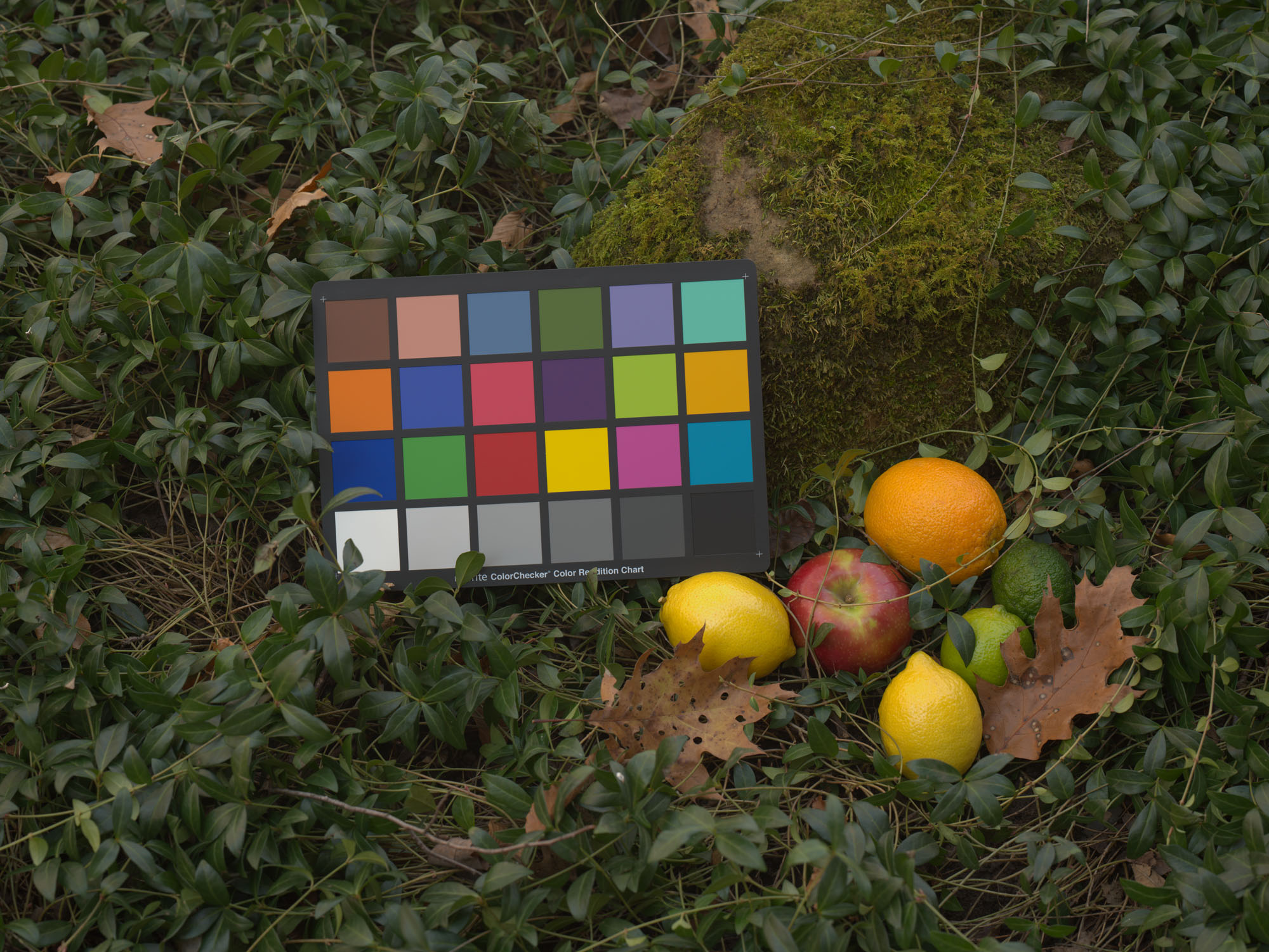
Figure 1. Image with color converted using the forward linear matrix discussed in the article.

Continue reading Linear Color: Applying the Forward Matrix →

ACR, Color, LR, Perceptual, Processing

Color: Determining a Forward Matrix for Your Camera

December 7, 2016 Jack 35 Comments

We understand from the previous article that rendering color with Adobe DNG raw conversion essentially means mapping raw data in the form of $rgb$ triplets into a standard color space via a Profile Connection Space in a two step process

$Raw Data \rightarrow XYZ_{D50} \rightarrow RGB_{standard}$

The first step white balances and demosaics the raw data, which at that stage we will refer to as $rgb$ , followed by converting it to $XYZ_{D50}$ Profile Connection Space through linear projection by an unknown ‘Forward Matrix’ (as DNG calls it) of the form

(1) $\begin{equation*} \left[ \begin{array}{c} X_{D50} \\ Y_{D50} \\ Z_{D50} \end{array} \right] = \begin{bmatrix} a_{11} & a_{12} & a_{13} \\ a_{21} & a_{22} & a_{23} \\ a_{31} & a_{32} & a_{33} \end{bmatrix} \left[ \begin{array}{c} r \\ g \\ b \end{array} \right] \end{equation*}$

with data as column-vectors in a 3xN array. Determining the nine $a$ coefficients of this matrix $M$ is the main subject of this article^[1]. Continue reading Color: Determining a Forward Matrix for Your Camera →

Color, Perceptual, Photometry, Processing, Radiometry

Color: From Object to Eye

December 4, 2016 Jack Leave a comment

How do we translate captured image information into a stimulus that will produce the appropriate perception of color? It’s actually not that complicated^[1].

Recall from the introductory article that a photon absorbed by a cone type ( $\rho$ , $\gamma$ or $\beta$ ) in the fovea produces the same stimulus to the brain regardless of its wavelength^[2]. Take the example of the eye of an observer which focuses on the retina the image of a uniform object with a spectral photon distribution of 1000 photons/nm in the 400 to 720nm wavelength range and no photons outside of it.

Because the system is linear, cones in the foveola will weigh the incoming photons by their relative sensitivity (probability) functions and add the result up to produce a stimulus proportional to the area under the curves. For instance a $\gamma$ cone may see about 321,000 photons arrive and produce a relative stimulus of about 94,700, the weighted area under the curve:

equal-photons-per-wl — Figure 1. Light made up of 321k photons of broad spectrum and constant Spectral Photon Distribution between 400 and 720nm is weighted by cone sensitivity to produce a relative stimulus equivalent to 94,700 photons, proportional to the area under the curve

Continue reading Color: From Object to Eye →

Color, Exposure, Perceptual, Photometry, Radiometry

An Introduction to Color in Digital Cameras

November 27, 2016 Jack 2 Comments

This article will set the stage for a discussion on how pleasing color is produced during raw conversion. The easiest way to understand how a camera captures and processes ‘color’ is to start with an example of how the human visual system does it.

An Example: Green

Light from the sun strikes leaves on a tree. The foliage of the tree absorbs some of the light and reflects the rest diffusely towards the eye of a human observer. The eye focuses the image of the foliage onto the retina at its back. Near the center of the retina there is a small circular area called fovea centralis which is dense with light receptors of well defined spectral sensitivities called cones. Information from the cones is pre-processed by neurons and carried by nerve fibers via the optic nerve to the brain where, after some additional psychovisual processing, we recognize the color of the foliage as green^[1].

spd-to-cone-quanta3 — Figure 1. The human eye absorbs light from an illuminant reflected diffusely by the object it is looking at.

Continue reading An Introduction to Color in Digital Cameras →

adobe camera raw, Color, LR, Processing, Sharpening

How Is a Raw Image Rendered?

October 21, 2016 Jack 19 Comments

What are the basic low level steps involved in raw file conversion? In this article I will discuss what happens under the hood of digital camera raw converters in order to turn raw file data into a viewable image, a process sometimes referred to as ‘rendering’. We will use the following raw capture by a Nikon D610 to show how image information is transformed at every step along the way:

Figure 1. Nikon D610 with AF-S 24-120mm f/4 lens at 24mm f/8 ISO100, minimally rendered from raw by Octave/Matlab following the steps outlined in the article.

Rendering = Raw Conversion + Editing

Continue reading How Is a Raw Image Rendered? →

IQ, Optics, Sharpness, Spatial Resolution

Taking the Sharpness Model for a Spin – II

October 5, 2016 Jack Leave a comment

This post will continue looking at the spatial frequency response measured by MTF Mapper off slanted edges in DPReview.com raw captures and relative fits by the ‘sharpness’ model discussed in the last few articles. The model takes the physical parameters of the digital camera and lens as inputs and produces theoretical directional system MTF curves comparable to measured data. As we will see the model seems to be able to simulate these systems well – at least within this limited set of parameters.

The following fits refer to the green channel of a number of interchangeable lens digital camera systems with different lenses, pixel sizes and formats – from the current Medium Format 100MP champ to the 1/2.3″ 18MP sensor size also sometimes found in the best smartphones. Here is the roster with the cameras as set up:

Table 1. The cameras and lenses under test.

Continue reading Taking the Sharpness Model for a Spin – II →

Optics, Sharpness, Spatial Resolution

Taking the Sharpness Model for a Spin

October 4, 2016 Jack Leave a comment

The series of articles starting here outlines a model of how the various physical components of a digital camera and lens can affect the ‘sharpness’ – that is the spatial resolution – of the images captured in the raw data. In this one we will pit the model against MTF curves obtained through the slanted edge method^[1]from real world raw captures both with and without an anti-aliasing filter.

With a few simplifying assumptions, which include ignoring aliasing and phase, the spatial frequency response (SFR or MTF) of a photographic digital imaging system near the center can be expressed as the product of the Modulation Transfer Function of each component in it. For a current digital camera these would typically be the main ones:

(1) $\begin{equation*} MTF_{sys} = MTF_{lens} (\cdot MTF_{AA}) \cdot MTF_{pixel} \end{equation*}$

all in two dimensions Continue reading Taking the Sharpness Model for a Spin →

Optics, Sharpness, Spatial Resolution

A Simple Model for Sharpness in Digital Cameras – Polychromatic Light

September 21, 2016 Jack Leave a comment

We now know how to calculate the two dimensional Modulation Transfer Function of a perfect lens affected by diffraction, defocus and third order Spherical Aberration – under monochromatic light at the given wavelength and f-number. In digital photography however we almost never deal with light of a single wavelength. So what effect does an illuminant with a wide spectral power distribution, going through the color filter of a typical digital camera CFA before the sensor have on the spatial frequency responses discussed thus far?

Monochrome vs Polychromatic Light

Not much, it turns out. Continue reading A Simple Model for Sharpness in Digital Cameras – Polychromatic Light →

Optics, Sharpness, Spatial Resolution

A Simple Model for Sharpness in Digital Cameras – Spherical Aberrations

September 18, 2016 Jack 6 Comments

Spherical Aberration (SA) is one key component missing from our MTF toolkit for modeling an ideal imaging system’s ‘sharpness’ in the center of the field of view in the frequency domain. In this article formulas will be presented to compute the two dimensional Point Spread and Modulation Transfer Functions of the combination of diffraction, defocus and third order Spherical Aberration for an otherwise perfect lens with a circular aperture.

Spherical Aberrations result because most photographic lenses are designed with quasi spherical surfaces that do not necessarily behave ideally in all situations. For instance, they may focus light on systematically different planes depending on whether the respective ray goes through the exit pupil closer or farther from the optical axis, as shown below:

371px-spherical_aberration_2 — Figure 1. Top: an ideal spherical lens focuses all rays on the same focal point. Bottom: a practical lens with Spherical Aberration focuses rays that go through the exit pupil based on their radial distance from the optical axis. Image courtesy Andrei Stroe.

Continue reading A Simple Model for Sharpness in Digital Cameras – Spherical Aberrations →

Optics, Sharpness, Spatial Resolution

A Simple Model for Sharpness in Digital Cameras – Defocus

September 13, 2016 Jack 10 Comments

This series of articles has dealt with modeling an ideal imaging system’s ‘sharpness’ in the frequency domain. We looked at the effects of the hardware on spatial resolution: diffraction, sampling interval, sampling aperture (e.g. a squarish pixel), anti-aliasing OLPAF filters. The next two posts will deal with modeling typical simple imperfections related to the lens: defocus and spherical aberrations.

Defocus = OOF

Defocus means that the sensing plane is not exactly where it needs to be for image formation in our ideal imaging system: the image is therefore out of focus (OOF). Said another way, light from a point source would go through the lens but converge either behind or in front of the sensing plane, as shown in the following diagram, for a lens with a circular aperture:

Figure 1. Back Focus, In Focus, Front Focus. — Figure 1. Top to bottom: Back Focus, In Focus, Front Focus. To the right is how the relative PSF would look like on the sensing plane. Image under license courtesy of Brion.

Continue reading A Simple Model for Sharpness in Digital Cameras – Defocus →

Sharpness, Spatial Resolution

A Simple Model for Sharpness in Digital Cameras – AA

September 9, 2016 Jack 2 Comments

This article will discuss a simple frequency domain model for an AntiAliasing (or Optical Low Pass) Filter, a hardware component sometimes found in a digital imaging system^[1]. The filter typically sits just above the sensor and its objective is to block as much of the aliasing and moiré creating energy above the monochrome Nyquist spatial frequency while letting through as much as possible of the real image forming energy below that, hence the low-pass designation.

Downsizing Box 4X — Figure 1. The blue line indicates the pass through performance of an ideal anti-aliasing filter presented with an Airy PSF (Original): pass all spatial frequencies below Nyquist (0.5 c/p) and none above that. No filter has such ideal characteristics and if it did its hard edges would result in undesirable ringing in the image.

In consumer digital cameras it is often implemented by introducing one or two birefringent plates in the sensor’s filter stack. This is how Nikon shows it for one of its DSLRs:

d800-aa1 — Figure 2. Typical Optical Low Pass Filter implementation in a current Digital Camera, courtesy of Nikon USA (yellow displacement ‘d’ added).

Continue reading A Simple Model for Sharpness in Digital Cameras – AA →

Quantization, Sensors, Spatial Resolution

The Units of Discrete Fourier Transforms

May 16, 2016 Jack 9 Comments

This article is about specifying the units of the Discrete Fourier Transform of an image and the various ways that they can be expressed. This apparently simple task can be fiendishly unintuitive.

The image we will use as an example is the familiar Airy Pattern from the last few posts, at f/16 with light of mean 530nm wavelength. Zoomed in to the left in Figure 1; and as it looks in its 1024×1024 sample image to the right:

Airy Mesh and Intensity — Figure 1. Airy disc image I(x,y). Left, 1a, 3D representation, zoomed in. Right, 1b, as it would appear on the sensing plane (yes, the rings are there but you need to squint to see them).

Continue reading The Units of Discrete Fourier Transforms →

IQ, Optics, Sensors, Sharpness, Spatial Resolution

A Simple Model for Sharpness in Digital Cameras – Sampling & Aliasing

May 12, 2016 Jack 8 Comments

Having shown that our simple two dimensional MTF model is able to predict the performance of the combination of a perfect lens and square monochrome pixel with 100% Fill Factor we now turn to the effect of the sampling interval on spatial resolution according to the guiding formula:

(1) $\begin{equation*} MTF_{Sys2D} = \left|(\widehat{ PSF_{lens} }\cdot \widehat{PIX_{ap} })\right|_{pu}\ast\ast\: \delta\widehat{\delta_{pitch}} \end{equation*}$

The hats in this case mean the Fourier Transform of the relative component normalized to 1 at the origin ( $_{pu}$ ), that is the individual MTFs of the perfect lens PSF, the perfect square pixel and the delta grid; $**$ represents two dimensional convolution.

Sampling in the Spatial Domain

While exposed a pixel sees the scene through its aperture and accumulates energy as photons arrive. Below left is the representation of, say, the intensity that a star projects on the sensing plane, in this case resulting in an Airy pattern since we said that the lens is perfect. During exposure each pixel integrates (counts) the arriving photons, an operation that mathematically can be expressed as the convolution of the shown Airy pattern with a square, the size of effective pixel aperture, here assumed to have 100% Fill Factor. It is the convolution in the continuous spatial domain of lens PSF with pixel aperture PSF shown in Equation (2) of the first article in the series.

Sampling is then the product of an infinitesimally small Dirac delta function at the center of each pixel, the red dots below left, by the result of the convolution, producing the sampled image below right.

Footprint-PSF3 — Figure 1. Left, 1a: A highly zoomed (3200%) image of the lens PSF, an Airy pattern, projected onto the imaging plane where the sensor sits. Pixels shown outlined in yellow. A red dot marks the sampling coordinates. Right, 1b: The sampled image zoomed at 16000%, 5x as much, because in this example each pixel’s width is 5 linear units on the side.

Continue reading A Simple Model for Sharpness in Digital Cameras – Sampling & Aliasing →

Optics, Sensors, Sharpness, Spatial Resolution

A Simple Model for Sharpness in Digital Cameras – Diffraction and Pixel Aperture

May 11, 2016 Jack 9 Comments

Now that we know from the introductory article that the spatial frequency response of a typical perfect digital camera and lens (its Modulation Transfer Function) can be modeled simply as the product of the Fourier Transform of the Point Spread Function of the lens and pixel aperture, convolved with a Dirac delta grid at cycles-per-pixel pitch spacing

(1) $\begin{equation*} MTF_{Sys2D} = \left|\widehat{ PSF_{lens} }\cdot \widehat{PIX_{ap} }\right|_{pu}\ast\ast\: \delta\widehat{\delta_{pitch}} \end{equation*}$

we can take a closer look at each of those components ( $pu$ here indicating normalization to one at the origin). I used Matlab to generate the examples below but you can easily do the same with a spreadsheet. Continue reading A Simple Model for Sharpness in Digital Cameras – Diffraction and Pixel Aperture →

IQ, Optics, Sensors, Sharpness, Spatial Resolution, Uncategorized

A Simple Model for Sharpness in Digital Cameras – I

May 9, 2016 Jack Leave a comment

The next few posts will describe a linear spatial resolution model that can help a photographer better understand the main variables involved in evaluating the ‘sharpness’ of photographic equipment and related captures. I will show numerically that the combined spectral frequency response (MTF) of a perfect AAless monochrome digital camera and lens in two dimensions can be described as the magnitude of the normalized product of the Fourier Transform (FT) of the lens Point Spread Function by the FT of the pixel footprint (aperture), convolved with the FT of a rectangular grid of Dirac delta functions centered at each pixel:

$MTF_{2D} = \left|\widehat{ PSF_{lens} }\cdot \widehat{PIX_{ap} }\right|_{pu}\ast\ast\: \delta\widehat{\delta_{pitch}}$

With a few simplifying assumptions we will see that the effect of the lens and sensor on the spatial resolution of the continuous image on the sensing plane can be broken down into these simple components. The overall ‘sharpness’ of the captured digital image can then be estimated by combining the ‘sharpness’ of each of them.

The stage will be set in this first installment with a little background and perfect components. Later additional detail will be provided to take into account pixel aperture and Anti-Aliasing filters. Then we will look at simple aberrations. Next we will learn how to measure MTF curves for our equipment, and look at numerical methods to model PSFs and MTFs from the wavefront at the aperture. Continue reading A Simple Model for Sharpness in Digital Cameras – I →

Optics, Spatial Resolution, USM

Chromatic Aberrations MTF Mapped

March 19, 2016 Jack Leave a comment

A number of interesting insights come to light once one realizes that as far as the slanted edge method (of measuring the Modulation Transfer Function of a Bayer CFA digital camera and lens from its raw data) is concerned it is as if it were dealing with identical images behind three color filters, each in their own separate, full resolution color plane:

CFA Sensor Frequency Domain Model — Figure 1. The Modulation Transfer Function of the three color planes can be measured separately directly in the raw data by open source MTF Mapper

Continue reading Chromatic Aberrations MTF Mapped →

IQ, MTF, Perceptual, PSF, Spatial Resolution, spectral response

COMBINING BAYER CFA MTF Curves – II

March 16, 2016 Jack 1 Comment

In this and the previous article I discuss how Modulation Transfer Functions (MTF) obtained from every color channel of a Bayer CFA raw capture in isolation can be combined to provide a meaningful composite MTF curve for the imaging system as a whole.

There are two ways that this can be accomplished: an input-referred approach ( $L$ ) that reflects the performance of the hardware only; and an output-referred one ( $Y$ ) that also takes into consideration how the image will be displayed. Both are valid and differences are typically minor, though the weights of the latter are scene, camera/lens, illuminant dependent – while the former are not. Therefore my recommendation in this context is to stick with input-referred weights when comparing cameras and lenses.¹ Continue reading COMBINING BAYER CFA MTF Curves – II →

IQ, Perceptual, Spatial Resolution

Combining Bayer CFA Modulation Transfer Functions – I

March 14, 2016 Jack Leave a comment

In this and the following article I will discuss my thoughts on how MTF50 results obtained from raw data of the four Bayer CFA color channels off a neutral target captured with a typical camera through the slanted edge method can be combined to provide a meaningful composite MTF50 for the imaging system as a whole. The perimeter of the discussion are neutral slanted edge measurements of Bayer CFA raw data for linear spatial resolution (‘sharpness’) photographic hardware evaluations. Corrections, suggestions and challenges are welcome. Continue reading Combining Bayer CFA Modulation Transfer Functions – I →

Color, IQ, Perceptual, Spatial Resolution, Uncategorized

Linearity in the Frequency Domain

March 12, 2016 Jack Leave a comment

For the purposes of ‘sharpness’ spatial resolution measurement in photography cameras can be considered shift-invariant, linear systems when capturing scene detail of random size and direction such as one often finds in landscapes.

Shift invariant means that the imaging system should respond exactly the same way no matter where light from the scene falls on the sensing medium . We know that in a strict sense this is not true because for instance pixels tend to have squarish active areas so their response cannot be isotropic by definition. However when using the slanted edge method of linear spatial resolution measurement we can effectively make it shift invariant by careful preparation of the testing setup. For example the edges should be slanted no more than this and no less than that. Continue reading Linearity in the Frequency Domain →

Information Science, IQ, Quantization, Sensors

Sub Bit Signal

January 19, 2016 Jack Leave a comment

My camera has a 14-bit ADC. Can it accurately record information lower than 14 stops below full scale? Can it store sub-LSB signals in the raw data?

With a well designed sensor the answer, unsurprisingly if you’ve followed the last few posts, is yes it can. The key to being able to capture such tiny visual information in the raw data is a well behaved imaging system with a properly dithered ADC. Continue reading Sub Bit Signal →

Posterization, Quantization

Sub LSB Quantization

October 8, 2015 Jack 3 Comments

This article is a little esoteric so one may want to skip it unless one is interested in the underlying mechanisms that cause quantization error as photographic signal and noise approach the darkest levels of acceptable dynamic range in our digital cameras: one least significant bit in the raw data. We will use our simplified camera model and deal with Poissonian Signal and Gaussian Read Noise separately – then attempt to bring them together.

Continue reading Sub LSB Quantization →

Quantization, Sensors

Photographic Sensor Simulation

September 22, 2015 Jack Leave a comment

Physicists and mathematicians over the last few centuries have spent a lot of their time studying light and electrons, the key ingredients of digital photography. In so doing they have left us with a wealth of theories to explain their behavior in nature and in our equipment. In this article I will describe how to simulate the information generated by a uniformly illuminated imaging system using open source Octave (or equivalently Matlab) utilizing some of these theories.

Since as you will see the simulations are incredibly (to me) accurate, understanding how the simulator works goes a long way in explaining the inner workings of a digital sensor at its lowest levels; and simulated data can be used to further our understanding of photographic science without having to run down the shutter count of our favorite SLRs. This approach is usually referred to as Monte Carlo simulation.

Continue reading Photographic Sensor Simulation →

Banding, Information Science, IQ, Perceptual, Posterization, Quantization

Smooth Gradients and the Weber-Fechner Fraction

September 15, 2015 Jack Leave a comment

Whether the human visual system perceives a displayed slow changing gradient of tones, such as a vast expanse of sky, as smooth or posterized depends mainly on two well known variables: the Weber-Fechner Fraction of the ‘steps’ in the reflected/produced light intensity (the subject of this article); and spatial dithering of the light intensity as a result of noise (the subject of a future one).

Continue reading Smooth Gradients and the Weber-Fechner Fraction →

Information Science, IQ, Sensors

Information Transfer: Non ISO-Invariant Case

June 15, 2015 Jack 21 Comments

We’ve seen how information about a photographic scene is collected in the ISOless/invariant range of a digital camera sensor, amplified, converted to digital data and stored in a raw file. For a given Exposure the best information quality (IQ) about the scene is available right at the photosites, only possibly degrading from there – but a properly designed** fully ISO invariant imaging system is able to store it in its entirety in the raw data. It is able to do so because the information carrying capacity (photographers would call it the dynamic range) of each subsequent stage is equal to or larger than the previous one. Cameras that are considered to be (almost) ISOless from base ISO include the Nikon D7000, D7200 and the Pentax K5. All digital cameras become ISO invariant above a certain ISO, the exact value determined by design compromises.

ToneTransferISOless100 — Figure 1: Simplified Scene Information Transfer in an ISO Invariant Imaging System at base ISO

In this article we’ll look at a class of imagers that are not able to store the whole information available at the photosites in one go in the raw file for a substantial portion of their working ISOs. The photographer can in such a case choose out of the full information available at the photosites what smaller subset of it to store in the raw data by the selection of different in-camera ISOs. Such cameras are sometimes improperly referred to as ISOful. Most Canon DSLRs fall into this category today. As do kings of darkness such as the Sony a7S or Nikon D5.

Continue reading Information Transfer: Non ISO-Invariant Case →

Banding, Information Science, IQ, Perceptual, Processing, Quantization, Sensors, Sharpening, USM

Image Quality: Raising ISO vs Pushing in Conversion

June 11, 2015 Jack 2 Comments

In the last few posts I have made the case that Image Quality in a digital camera is entirely dependent on the light Information collected at a sensor’s photosites during Exposure. Any subsequent processing – whether analog amplification and conversion to digital in-camera and/or further processing in-computer – effectively applies a set of Information Transfer Functions to the signal that when multiplied together result in the data from which the final photograph is produced. Each step of the way can at best maintain the original Information Quality (IQ) but in most cases it will degrade it somewhat.

IQ: Only as Good as at Photosites’ Output

This point is key: in a well designed imaging system** the final image IQ is only as good as the scene information collected at the sensor’s photosites, independently of how this information is stored in the working data along the processing chain, on its way to being transformed into a pleasing photograph. As long as scene information is properly encoded by the system early on, before being written to the raw file – and information transfer is maintained in the data throughout the imaging and processing chain – final photograph IQ will be virtually the same independently of how its data’s histogram looks along the way.

Continue reading Image Quality: Raising ISO vs Pushing in Conversion →

Banding, Information Science, IQ

The Difference Between Data and Information

June 10, 2015 Jack Leave a comment

In photography, digital cameras capture information about the scene carried by photons reflected by it and store the information as data in a raw file pretty well linearly. Data is the container, scene information is the substance. There may or may not be information in the data, no matter what its form. With a few limitations what counts is the substance, information, not the form, data.

A Simple Example

Imagine for instance that you are taking stock of the number of remaining pieces in your dinner place settings. You originally had a full set of 6 of everything but today, after many years of losses and breakage, this is the situation in each category: Continue reading The Difference Between Data and Information →

Exposure, Information Science, IQ, Uncategorized

Information Transfer – The ISO Invariant Case

June 8, 2015 Jack 6 Comments

We know that the best Information Quality possible collected from the scene by a digital camera is available right at the output of the sensor and it will only be degraded from there. This article will discuss what happens to this information as it is transferred through the imaging system and stored in the raw data. It will use the simple language outlined in the last post to explain how and why the strategy for Capturing the best Information or Image Quality (IQ) possible from the scene in the raw data involves only two simple steps:

1) Maximizing the collected Signal given artistic and technical constraints; and
2) Choosing what part of the Signal to store in the raw data and what part to leave behind.

The second step is only necessary if your camera is incapable of storing the entire Signal at once (that is it is not ISO invariant) and will be discussed in a future article. In this post we will assume an ISOless imaging system.

Continue reading Information Transfer – The ISO Invariant Case →

Information Science, IQ, Sensors

Information Theory for Photographers

May 21, 2015 Jack Leave a comment

Ever since Einstein we’ve been able to say that humans ‘see’ because information about the scene is carried to the eyes by photons reflected by it. So when we talk about Information in photography we are referring to information about the energy and distribution of photons arriving from the scene. The more complete this information, the better we ‘see’. No photons = no information = no see; few photons = little information = see poorly = poor IQ; more photons = more information = see better = better IQ.

Sensors in digital cameras work similarly, their output ideally being the energy and location of every photon incident on them during Exposure. That’s the full information ideally required to recreate an exact image of the original scene for the human visual system, no more and no less. In practice however we lose some of this information along the way during sensing, so we need to settle for approximate location and energy – in the form of photoelectron counts by pixels of finite area, often correlated to a color filter array.

Continue reading Information Theory for Photographers →

Information Science, IQ, Quantization, Sensors

How Many Bits to Fully Encode My Image

May 19, 2015 Jack 2 Comments

My camera sports a 14 stop Engineering Dynamic Range. What bit depth do I need to safely fully encode all of the captured tones from the scene with a linear sensor? As we will see the answer is not 14 bits because that’s the eDR, but it’s not too far from that either – for other reasons, as information science will show us in this article.

When photographers talk about grayscale ‘tones’ they typically refer to the number of distinct gray levels present in a displayed image. They don’t want to see distinct levels in a natural slow changing gradient like a dark sky: if it’s smooth they want to perceive it as smooth when looking at their photograph. So they want to make sure that all possible tonal information from the scene has been captured and stored in the raw data by their imaging system.

Continue reading How Many Bits to Fully Encode My Image →

IQ, Sensors

Dynamic Range and Bit Depth

May 15, 2015 Jack 4 Comments

My camera has an engineering Dynamic Range of 14 stops, how many bits do I need to encode that DR? Well, to encode the whole Dynamic Range 1 bit could suffice, depending on the content and the application. The reason is simple, dynamic range is only concerned with the extremes, not with tones in between:

$DR = \frac{Maximum Signal}{Minimum Signal}$

So in theory we only need 1 bit to encode it: zero for minimum signal and one for maximum signal, like so

Continue reading Dynamic Range and Bit Depth →

IQ, Sensors

Engineering Dynamic Range in Photography

May 13, 2015 Jack Leave a comment

Dynamic Range (DR) in Photography usually refers to the linear working signal range, from darkest to brightest, that the imaging system is capable of capturing and/or displaying. It is expressed as a ratio, in stops:

$DR = log_2(\frac{Maximum Acceptable Signal}{Minimum Acceptable Signal})$

It is a key Image Quality metric because photography is all about contrast, and dynamic range limits the range of recordable/ displayable tones. Different components in the imaging system have different working dynamic ranges and the system DR is equal to the dynamic range of the weakest performer in the chain.

Continue reading Engineering Dynamic Range in Photography →

Deconvolution, IQ, Sharpening, Spatial Resolution

Downsizing Algorithms: Effects on Resolution

April 8, 2015 Jack 3 Comments

Most of the photographs captured these days end up being viewed on a display of some sort, with at best 4K (4096×2160) but often no better than HD resolution (1920×1080). Since the cameras that capture them have typically several times that number of pixels, 6000×4000 being fairly normal today, most images need to be substantially downsized for viewing, even allowing for some cropping. Resizing algorithms built into browsers or generic image viewers tend to favor expediency over quality, so it behooves the IQ conscious photographer to manage the process, choosing the best image size and downsampling algorithm for the intended file and display medium.

When downsizing the objective is to maximize the original spatial resolution retained while minimizing the possibility of aliasing and moirè. In this article we will take a closer look at some common downsizing algorithms and their effect on spatial resolution information in the frequency domain.

Continue reading Downsizing Algorithms: Effects on Resolution →

Deconvolution, Processing, Sharpening, Spatial Resolution

Raw Converter Sharpening with Sliders at Zero?

April 7, 2015 Jack 9 Comments

I’ve mentioned in the past that I prefer to take spatial resolution measurements directly off the raw information in order to minimize often unknown subjective variables introduced by demosaicing and rendering algorithms unbeknownst to the operator, even when all relevant sliders are zeroed. In this post we discover that that is indeed the case for ACR/LR process 2010/2012 and for Capture NX-D – while DCRAW appears to be transparent and perform straight out demosaicing with no additional processing without the operator’s knowledge.

Continue reading Raw Converter Sharpening with Sliders at Zero? →

Equivalence, Formats, IQ, Spatial Resolution

Are micro Four Thirds Lenses Typically Twice as ‘Sharp’ as Full Frame’s?

March 30, 2015 Jack 4 Comments

In fact the question is more generic than that. Smaller format lens designers try to compensate for their imaging system geometric resolution penalty (compared to a larger format when viewing final images at the same size) by designing ‘sharper’ lenses specifically for it, rather than recycling larger formats’ designs (feeling guilty APS-C?) – sometimes with excellent effect. Are they succeeding? I will use mFT only as an example here, but input is welcome for all formats, from phones to large format.

Continue reading Are micro Four Thirds Lenses Typically Twice as ‘Sharp’ as Full Frame’s? →

IQ, Sensors

Determining Sensor IQ Metrics: RN, FWC, PRNU, DR, gain – 2

March 6, 2015 Jack 2 Comments

There are several ways to extract Sensor IQ metrics like read noise, Full Well Count, PRNU, Dynamic Range and others from mean and standard deviation statistics obtained from a uniform patch in a camera’s raw file. In the last post we saw how to do it by using such parameters to make observed data match the measured SNR curve. In this one we will achieve the same objective by fitting mean and standard deviation data. Since the measured data is identical, if the fit is good so should be the results.

Sensor Metrics from Measured Mean and Standard Deviation in DN

Continue reading Determining Sensor IQ Metrics: RN, FWC, PRNU, DR, gain – 2 →

IQ, Sensors

Determining Sensor IQ Metrics: RN, FWC, PRNU, DR, gain – 1

March 5, 2015 Jack Leave a comment

We’ve seen how to model sensors and how to collect signal and noise statistics from the raw data of our digital cameras. In this post I am going to pull both things together allowing us to estimate sensor IQ metrics: input-referred read noise, clipping/saturation/Full Well Count, Dynamic Range, Pixel Response Non-Uniformities and gain/sensitivity.

There are several ways to extract these metrics from signal and noise data obtained from a camera’s raw file. I will show two related ones: via SNR in this post and via total noise N in the next. The procedure is similar and the results are identical.

Continue reading Determining Sensor IQ Metrics: RN, FWC, PRNU, DR, gain – 1 →

IQ, Sensors

Sensor IQ’s Simple Model

March 4, 2015 Jack Leave a comment

Imperfections in an imaging system’s capture process manifest themselves in the form of deviations from the expected signal. We call these imperfections ‘noise’ because they introduce grain and artifacts in our images. The fewer the imperfections, the lower the noise, the higher the image quality.

However, because the Human Visual System is adaptive within its working range, it’s not the absolute amount of noise that matters to perceived Image Quality (IQ) as much as the amount of noise relative to the signal – represented for instance by the Signal to Noise Ratio (SNR). That’s why to characterize the performance of a sensor in addition to signal and noise we also need to determine its sensitivity and the maximum signal it can detect.

In this series of articles I will describe how to use the Photon Transfer method and a spreadsheet to determine basic IQ performance metrics of a digital camera sensor. It is pretty easy if we keep in mind the simple model of how light information is converted into raw data by digital cameras:

Continue reading Sensor IQ’s Simple Model →

Spatial Resolution

MTF Mapper vs sfrmat3

February 13, 2015 Jack 3 Comments

Over the last couple of years I’ve been using Frans van den Bergh‘s excellent open source MTF Mapper to measure the Modulation Transfer Function of imaging systems off a slanted edge target, as you may have seen in these pages. As long as one understands how to get the most out of it I find it a solid product that gives reliable results, with MTF50 typically well within 2% of actual in less than ideal real-world situations (see below). I had little to compare it to other than to tests published by gear testing sites: they apparently mostly use a commercial package called Imatest for their slanted edge readings – and it seemed to correlate well with those.

Then recently Jim Kasson pointed out sfrmat3, the matlab program written by Peter Burns who is a slanted edge method expert who worked at Kodak and was a member of the committee responsible for ISO12233, the resolution and spatial frequency response standard for photography. sfrmat3 is considered to be a solid implementation of the standard and many, including Imatest, benchmark against it – so I was curious to see how MTF Mapper 0.4.1.6 would compare. It did well.

Continue reading MTF Mapper vs sfrmat3 →

Equivalence, Formats, IQ, Perceptual, Sharpening, Spatial Resolution

Can MTF50 be Trusted?

February 10, 2015 Jack 2 Comments

A reader suggested that a High-Res Olympus E-M5 Mark II image used in the previous post looked sharper than the equivalent Sony a6000 image, contradicting the relative MTF50 measurements, perhaps showing ‘the limitations of MTF50 as a methodology’. That would be surprising because MTF50 normally correlates quite well with perceived sharpness, so I decided to check this particular case out.

‘Who are you going to believe, me or your lying eyes’?

Continue reading Can MTF50 be Trusted? →

Equivalence, Formats, IQ, Sensors, Spatial Resolution

Olympus E-M5 II High-Res 64MP Shot Mode

February 6, 2015 Jack 21 Comments

Olympus just announced the E-M5 Mark II, an updated version of its popular micro Four Thirds E-M5 model, with an interesting new feature: its 16MegaPixel sensor, presumably similar to the one in other E-Mx bodies, has a high resolution mode where it gets shifted around by the image stabilization servos during exposure to capture, as they say in their press release

‘resolution that goes beyond full-frame DSLR cameras. 8 images are captured with 16-megapixel image information while moving the sensor by 0.5 pixel steps between each shot. The data from the 8 shots are then combined to produce a single, super-high resolution image, equivalent to the one captured with a 40-megapixel image sensor.’

A great idea that could give a welcome boost to the ‘sharpness’ of this handy system. Preliminary tests show that the E-M5 mk II 64MP High-Res mode gives some advantage in MTF50 linear spatial resolution compared to the Standard Shot 16MP mode with the captures in this post. Plus it apparently virtually eliminates the possibility of aliasing and moiré. Great stuff, Olympus.

Continue reading Olympus E-M5 II High-Res 64MP Shot Mode →

Equivalence, Formats, IQ, Sensors, Spatial Resolution

Equivalence in Pictures: Sharpness/Spatial Resolution

February 4, 2015 Jack 8 Comments

So, is it true that a Four Thirds lens needs to be about twice as ‘sharp’ as its Full Frame counterpart in order to be able to display an image of spatial resolution equivalent to the larger format’s?

It is, because of the simple geometry I will describe in this article. In fact with a few provisos one can generalize and say that lenses from any smaller format need to be ‘sharper’ by the ratio of their sensor diagonals in order to produce the same linear resolution on same-sized final images.

This is one of the reasons why Ansel Adams shot 4×5 and 8×10 – and I would too, were it not for logistical and pecuniary concerns.

Continue reading Equivalence in Pictures: Sharpness/Spatial Resolution →

Equivalence, Formats, Sensors

Equivalence in Pictures: Focal Length, f-number, diffraction, DOF

January 31, 2015 Jack Leave a comment

Equivalence – as we’ve discussed one of the fairest ways to compare the performance of two cameras of different physical formats, characteristics and specifications – essentially boils down to two simple realizations for digital photographers:

metrics need to be expressed in units of picture height (or diagonal where the aspect ratio is significantly different) in order to easily compare performance with images displayed at the same size; and
focal length changes proportionally to sensor size in order to capture identical scene content on a given sensor, all other things being equal.

The first realization should be intuitive (see next post). The second one is the subject of this post: I will deal with it through a couple of geometrical diagrams.

Continue reading Equivalence in Pictures: Focal Length, f-number, diffraction, DOF →

Equivalence, IQ, Optics, Sensors, Spatial Resolution

The Units of Spatial Resolution

January 23, 2015 Jack 15 Comments

Several sites for photographers perform spatial resolution ‘sharpness’ testing of a specific lens and digital camera set up by capturing a target. You can also measure your own equipment relatively easily to determine how sharp your hardware is. However comparing results from site to site and to your own can be difficult and/or misleading, starting from the multiplicity of units used: cycles/pixel, line pairs/mm, line widths/picture height, line pairs/image height, cycles/picture height etc.

This post will address the units involved in spatial resolution measurement using as an example readings from the popular slanted edge method, although their applicability is generic.

Continue reading The Units of Spatial Resolution →

Exposure, IQ, Sensors, Uncategorized

How to Measure the SNR Performance of Your Digital Camera

January 22, 2015 Jack 1 Comment

Determining the Signal to Noise Ratio (SNR) curves of your digital camera at various ISOs and extracting from them the underlying IQ metrics of its sensor can help answer a number of questions useful to photography. For instance whether/when to raise ISO; what its dynamic range is; how noisy its output could be in various conditions; or how well it is likely to perform compared to other Digital Still Cameras. As it turns out obtaining the relative data is a little time consuming but not that hard. All you need is your camera, a suitable target, a neutral density filter, dcraw or libraw or similar software to access the linear raw data – and a spreadsheet.

Continue reading How to Measure the SNR Performance of Your Digital Camera →

Equivalence, Exposure, Formats, IQ, Sensors

Comparing Sensor SNR

October 11, 2014 Jack 4 Comments

We’ve seen how SNR curves can help us analyze digital camera IQ:

In this post we will use them to help us compare digital cameras, independently of format size. Continue reading Comparing Sensor SNR →

IQ, Sensors

SNR Curves and IQ in Digital Cameras

October 8, 2014 Jack 1 Comment

In photography the higher the ratio of Signal to Noise, the less grainy the final image normally looks. The Signal-to-Noise-ratio SNR is therefore a key component of Image Quality. Let’s take a closer look at it. Continue reading SNR Curves and IQ in Digital Cameras →

IQ, Sensors

The Difference between Peak and Effective Quantum Efficiency

October 6, 2014 Jack Leave a comment

Effective Quantum Efficiency as I calculate it is an estimate of the probability that a visible photon – from a ‘Daylight’ blackbody radiating source at a temperature of 5300K impinging on the sensor in question after making it through its IR filter, UV filter, AA low pass filter, microlenses, average Color Filter – will produce a photoelectron upon hitting silicon:

(1) $\begin{equation*} EQE = \frac{n_{e^-} \text{ produced by average pixel}}{n_{ph} \text{ incident on average pixel}} \end{equation*}$

with $n_{e^-}$ the signal in photoelectrons and $n_{ph}$ the number of photons incident on the sensor at the given Exposure as shown below. Continue reading The Difference between Peak and Effective Quantum Efficiency →

Equivalence, Exposure, IQ, Sensors

Equivalence and Equivalent Image Quality: Signal

October 4, 2014 Jack 1 Comment

One of the fairest ways to compare the performance of two cameras of different physical characteristics and specifications is to ask a simple question: which photograph would look better if the cameras were set up side by side, captured identical scene content and their output were then displayed and viewed at the same size?

Achieving this set up and answering the question is anything but intuitive because many of the variables involved, like depth of field and sensor size, are not those we are used to dealing with when taking photographs. In this post I would like to attack this problem by first estimating the output signal of different cameras when set up to capture Equivalent images.

It’s a bit long so I will give you the punch line first: digital cameras of the same generation set up equivalently will typically generate more or less the same signal in $e^-$ independently of format. Ignoring noise, lenses and aspect ratio for a moment and assuming the same camera gain and number of pixels, they will produce identical raw files. Continue reading Equivalence and Equivalent Image Quality: Signal →

IQ, Spatial Resolution

How to Get MTF Performance Curves for Your Camera and Lens

October 3, 2014 Jack Leave a comment

You have obtained a raw file containing the image of a slanted edge captured with good technique. How do you get the Modulation Transfer Function of the camera and lens combination that took it? Download and feast your eyes on open source MTF Mapper version 0.4.16 by Frans van den Bergh.

[Edit, several years later: MTF Mapper has kept improving over time, making it in my opinion the most accurate slanted edge measuring tool available today, used in applications that range from photography to machine vision to the Mars Rover. Did I mention that it is open source?

It now sports a Graphical User Interface which can load raw files and allow the arbitrary selection of individual edges by simply pointing and clicking, making this post largely redundant. The procedure outlined will still work but there are easier ways to accomplish the same task today. To obtain the same result with raw data and version 0.7.38 just install MTF Mapper, set the “Settings/Preferences” tab as follows and leave all else at default:

“Pixel size” is only needed to also show SFR in units of lp/mm and the “Arguments” field only if using an unspecified raw data CFA layout. “Accept” and “File/Open with manual edge selection” your raw files. Follow the instructions to select as many edges as desired. Then in “Data set” open an “annotated” file and shift-click on the chosen edges to see the relative MTF plots.]

The first thing we are going to do is crop the edges and package them into a TIFF file format so that MTF Mapper has an easier time reading them. Let’s use as an example a Nikon D810+85mm:1.8G ISO 64 studio raw capture by DPReview so that you can follow along if you wish. Continue reading How to Get MTF Performance Curves for Your Camera and Lens →

IQ, Optics, Sharpness, Spatial Resolution

The Slanted Edge Method

October 2, 2014 Jack 25 Comments

My preferred method for measuring the spatial resolution performance of photographic equipment these days is the slanted edge method. It requires a minimum amount of additional effort compared to capturing and simply eye-balling a pinch, Siemens or other chart but it gives more, useful, accurate, quantitative information in the language and units that have been used to characterize optical systems for over a century: it produces a good approximation to the Modulation Transfer Function of the two dimensional camera/lens system impulse response – at the location of the edge in the direction perpendicular to it.

Much of what there is to know about an imaging system’s spatial resolution performance can be deduced by analyzing its MTF curve, which represents the system’s ability to capture increasingly fine detail from the scene, starting from perceptually relevant metrics like MTF50, discussed a while back.

In fact the area under the curve weighted by some approximation of the Contrast Sensitivity Function of the Human Visual System is the basis for many other, better accepted single figure ‘sharpness‘ metrics with names like Subjective Quality Factor (SQF), Square Root Integral (SQRI), CMT Acutance, etc. And all this simply from capturing the image of a slanted edge, which one can actually and somewhat easily do at home, as presented in the next article.

Continue reading The Slanted Edge Method →

IQ, Perceptual, Sharpening, Spatial Resolution

Why Raw Sharpness IQ Measurements Are Better

October 2, 2014 Jack Leave a comment

Why Raw? The question is whether one is interested in measuring the objective, quantitative spatial resolution capabilities of the hardware or whether instead one would prefer to measure the arbitrary, qualitatively perceived sharpening prowess of (in-camera or in-computer) processing software as it turns the capture into a pleasing final image. Either is of course fine.

My take on this is that the better the IQ captured the better the final image will be after post processing. In other words I am typically more interested in measuring the spatial resolution information produced by the hardware comfortable in the knowledge that if I’ve got good quality data to start with its appearance will only be improved in post by the judicious use of software. By IQ here I mean objective, reproducible, measurable physical quantities representing the quality of the information captured by the hardware, ideally in scientific units.

Can we do that off a file rendered by a raw converter or, heaven forbid, a Jpeg? Not quite, especially if the objective is measuring IQ. Continue reading Why Raw Sharpness IQ Measurements Are Better →

IQ, Perceptual, Sharpening, Spatial Resolution

How Sharp are my Camera and Lens?

October 1, 2014 Jack Leave a comment

You want to measure how sharp your camera/lens combination is to make sure it lives up to its specs. Or perhaps you’d like to compare how well one lens captures spatial resolution compared to another you own. Or perhaps again you are in the market for new equipment and would like to know what could be expected from the shortlist. Or an old faithful is not looking right and you’d like to check it out. So you decide to do some testing. Where to start?

In the next four articles I will walk you through my methodology based on captures of slanted edge targets:

Continue reading How Sharp are my Camera and Lens? →

Exposure, Sensors

What is the Effective Quantum Efficiency of my Sensor?

September 23, 2014 Jack Leave a comment

Now that we know how to determine how many photons impinge on a sensor we can estimate its Effective Quantum Efficiency, that is the efficiency with which it turns such a photon flux ( $n_{ph}$ ) into photoelectrons ( $n_{e^-}$ ), which will then be converted to raw data to be stored in the capture’s raw file:

(1) $\begin{equation*} EQE = \frac{n_{e^-} \text{ produced by average pixel}}{n_{ph} \text{ incident on average pixel}} \end{equation*}$

I call it ‘Effective’, as opposed to ‘Absolute’, because it represents the probability that a photon arriving on the sensing plane from the scene will be converted to a photoelectron by a given pixel in a digital camera sensor. It therefore includes the effect of microlenses, fill factor, CFA and other filters on top of silicon in the pixel. Whether Effective or Absolute, QE is usually expressed as a percentage, as seen below in the specification sheet of the KAF-8300 by On Semiconductor, without IR/UV filters:

For instance if an average of 100 photons per pixel were incident on a uniformly lit spot on the sensor and on average each pixel produced a signal of 20 photoelectrons we would say that the Effective Quantum Efficiency of the sensor is 20%. Clearly the higher the EQE the better for Image Quality parameters such as SNR. Continue reading What is the Effective Quantum Efficiency of my Sensor? →

Banding, Perceptual, Quantization

I See Banding in the Sky. Is my Camera Faulty?

September 22, 2014 Jack Leave a comment

This is a recurring nightmare for a new photographer: they head out with their brand new state-of-the art digital camera, capture a set of images with a vast expanse of sky or smoothly changing background, come home, fire them up on their computer, play with a few sliders and … gasp! … there are visible bands (posterization, stairstepping, quantization) all over the smoothly changing gradient. ‘Is my new camera broken?!’, they wonder in horror.

Relax, chances are very (very) good that the camera is fine. I am going to show you in this post how to make sure that that is indeed the case and hone in on the real culprit(s). Continue reading I See Banding in the Sky. Is my Camera Faulty? →

Exposure, Photometry, Radiometry, Sensors

How Many Photons on a Pixel at a Given Exposure

September 22, 2014 Jack 2 Comments

How many photons impinge on a pixel illuminated by a known light source during exposure? To answer this question in a photographic context under daylight we need to know the effective area of the pixel, the Spectral Power Distribution of the illuminant and the relative Exposure.

We can typically estimate the pixel’s effective area and the Spectral Power Distribution of the illuminant – so all we need to determine is what Exposure the relative irradiance corresponds to in order to obtain the answer.

Continue reading How Many Photons on a Pixel at a Given Exposure →

Exposure, Radiometry

Photons Emitted by Light Source

September 16, 2014 Jack 6 Comments

How many photons are emitted by a light source? To answer this question we need to evaluate the following simple formula at every wavelength in the spectral range of interest and add the values up:

(1) $\begin{equation*} \frac{\text{Power of Light in }W/m^2}{\text{Energy of Average Photon in }J/photon} \end{equation*}$

The Power of Light emitted in $W/m^2$ is called Spectral Exitance, with the symbol $M_e(\lambda)$ when referred to units of energy. The energy of one photon at a given wavelength is

(2) $\begin{equation*} e_{ph}(\lambda) = \frac{hc}{\lambda}\text{ joules/photon} \end{equation*}$

with $\lambda$ the wavelength of light in meters and $h$ and $c$ Planck’s constant and the speed of light in the chosen medium respectively. Since Watts are joules per second the units of (1) are therefore $photons/m^2/s$ . Writing it more formally:

(3) $\begin{equation*} M_{ph} = \int\limits_{\lambda_1}^{\lambda_2} \frac{M_e(\lambda)\cdot \lambda \cdot d\lambda}{hc} \text{ $\frac{photons}{m^2\cdot s}$} \end{equation*}$

Continue reading Photons Emitted by Light Source →

Exposure, Perceptual, Photometry

Converting Radiometric to Photometric Units

September 16, 2014 Jack Leave a comment

When first approaching photographic science a photographer is often confused by the unfamiliar units used. In high school we were taught energy and power in radiometric units like watts ($W$) – while in photography the same concepts are dealt with in photometric units like lumens ($lm$).

Once one realizes that both sets of units refer to the exact same physical process – energy transfer – but they are fine tuned for two slightly different purposes it becomes a lot easier to interpret the science behind photography through the theory one already knows.

It all boils down to one simple notion: lumens are watts as perceived by the Human Visual System.

Continue reading Converting Radiometric to Photometric Units →

Exposure, Sensors

How Many Photons on a Pixel

September 10, 2014 Jack 2 Comments

How many visible photons hit a pixel on my sensor? The answer depends on Exposure, Spectral power distribution of the arriving light and effective pixel area. With a few simplifying assumptions it is not difficult to calculate that with a typical Daylight illuminant the number is roughly 11,760 photons per lx-s per $\mu m^2$ . Without the simplifying assumptions* it reduces to about 11,000. Continue reading How Many Photons on a Pixel →

Color, Photometry, Sensors

Nikon CFA Spectral Power Distribution

September 9, 2014 Jack 8 Comments

I measured the Spectral Photon Distribution of the three CFA filters of a Nikon D610 in ‘Daylight’ conditions with a cheap spectrometer. Taking a cue from this post I pointed it at light from the sun reflected off a gray card and took a raw capture of the spectrum it produced.

An ImageJ plot did the rest. I took a dozen captures at slightly different angles to catch the picture of the clearest spectrum. Shown are the three spectral curves averaged over the two best opposing captures, each proportional to the number of photons let through by the respective Color Filter. The units on the vertical axis are raw black-subtracted values from the raw file (DN), therefore the units on the vertical axis are proportional to the number of incident photons in each case. The Photopic Eye Luminous Efficiency Function (2 degree, Sharpe et al 2005) is also shown for reference, scaled to the same maximum as the green curve (although in energy units, my bad). Continue reading Nikon CFA Spectral Power Distribution →

Equivalence, Formats, Sensors

Focus Tolerance and Format Size

September 5, 2014 Jack Leave a comment

The key variable as far as the tolerances required to position the lens for accurate focus are concerned (at least in a simplified ideal situation) is an appropriate approximate distance between the desired in-focus plane and the actual in-focus plane (which we are assuming is slightly out of focus). It is a distance in the direction perpendicular to the x-y plane normally used to describe position of the image on it, hence the designation delta z, or dz in this post. The lens’ allowable focus tolerance is therefore +/- dz, which we will show in this post to vary as the square of the format’s diagonal. Continue reading Focus Tolerance and Format Size →

Perceptual, Sharpness, Spatial Resolution

MTF50 and Perceived Sharpness

September 5, 2014 Jack 7 Comments

Is MTF50 a good proxy for perceived sharpness? In this article and those that follow MTF50 indicates the spatial frequency at which the Modulation Transfer Function of an imaging system is half (50%) of what it would be if the system did not degrade detail in the image painted by incoming light.

It makes intuitive sense that the spatial frequencies that are most closely related to our perception of sharpness vary with the size and viewing distance of the displayed image.

For instance if an image captured by a Full Frame camera is viewed at ‘standard’ distance (that is a distance equal to its diagonal), it turns out that the portion of the MTF curve most representative of perceived sharpness appears to be around MTF90. On the other hand, when pixel peeping the spatial frequencies around MTF50 look to be a decent, simple to calculate indicator of it, assuming a well set up imaging system in good working conditions. Continue reading MTF50 and Perceived Sharpness →

Exposure, Information Science, IQ, Sensors

Exposure and ISO

September 5, 2014 Jack Leave a comment

The in-camera ISO dial is a ballpark milkshake of an indicator to help choose parameters that will result in a ‘good’ perceived picture. Key ingredients to obtain a ‘good’ perceived picture are 1) ‘good’ Exposure and 2) ‘good’ in-camera or in-computer processing. It’s easier to think about them as independent processes and that comes naturally to you because you shoot raw in manual mode and you like to PP, right? Continue reading Exposure and ISO →

White Point

Absolute Raw Data

An Example: Green

Rendering = Raw Conversion + Editing

Monochrome vs Polychromatic Light

Defocus = OOF

Sampling in the Spatial Domain

IQ: Only as Good as at Photosites’ Output

A Simple Example

Sensor Metrics from Measured Mean and Standard Deviation in DN

‘Who are you going to believe, me or your lying eyes’?

It all boils down to one simple notion: lumens are watts as perceived by the Human Visual System.

Musings about Photography