Physicists and mathematicians over the last few centuries have spent a lot of their time studying light and electrons, the key ingredients of digital photography. In so doing they have left us with a wealth of theories to explain their behavior in nature and in our equipment. In this article I will describe how to simulate the information generated by a uniformly illuminated imaging system using open source Octave (or equivalently Matlab) utilizing some of these theories.
Since as you will see the simulations are incredibly (to me) accurate, understanding how the simulator works goes a long way in explaining the inner workings of a digital sensor at its lowest levels; and simulated data can be used to further our understanding of photographic science without having to run down the shutter count of our favorite SLRs. This approach is usually referred to as Monte Carlo simulation.
A Digital Camera Model
Digital cameras are very complex devices, but their job can be described by a simple model as discussed in a previous article.
The simple model that we will use assumes that each pixel in the sensor is exposed to uniform light (photons) from the scene during a capture and generates a certain number of photoelectrons which are collected at the output of the pixel’s photodiode, then amplified, fed to an Analog to Digital Converter and stored in the raw file as Data Numbers. All random noise is assumed to be added at the output of the pixels* (the input to the electronics), before a perfect amplifier and ADC.

As described in the earlier article the amplification and conversion of photoelectrons (e-) and noise (e- rms) to data numbers in the raw file (DN) results in an effective system gain in units of DN/e-.
The Output of the Pixels* is Quantized
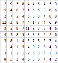
When a pixel is exposed to incident photons the photoelectric effect generates photoelectrons proportional to their number according to Poisson statistics of well known distribution around the mean. There never are negative counts. Thanks to quantum mechanics we know that the number of photoelectrons collected at the output of each pixel’s photodiode is an integer. There will never be 5.2 e- in the photodiode when it is read: there will be either 5, 6 or another discrete number. For instance if a given uniformly exposed capture produced a mean of 5.2e- per pixel, this is the number and distribution of photoelectrons that we could expect to see in each pixel (10×10 area shown):
The fluctuation of the signal about the mean is referred to as shot noise, and its standard deviation is the square root of the mean, as you can read in a dedicated article. In Octave/Matlab signal generation with a Poisson distribution in e- can be accomplished by the command
sensorOut_e = poissrnd(5.2,10,10); %units are e-
The 10×10 chart above was generated with that script. This is the histogram of a larger uniform area with a mean signal of 5.2 e-. The ‘bins’ can only be positive integers because photoelectron generation follows Poisson statistics.

Read Noise is Not
The input referred random read noise that is added to the integer e- count collected at each pixel sense node can instead be considered to be continuous. The model assumes it to be part of the analog circuitry and to come in a Normal distribution with a mean of zero, which means that it will produce both positive and negative values with decimal places, effectively in floating point notation. In Octave and Matlab read noise of standard deviation 3.0276e- for a 10×10 pixel area can be simulated by the function randn which generates a normal distribution in the range 0->1
readNoise_e = randn(10,10) * 3.0276; %units are e- rms
This is the histogram of a 200×200 uniform area of random noise only with a standard deviation of 3.0276 e-. The ‘bins’ are arbitrary since the underlying data is supposed to be ‘continuous’:

Gain is Continuous and ADC rounds
Pixel output plus the additive input referred read noise, both in units of e-, are then amplified by ISO-controlled analog gain and fed to the ADC for conversion to raw data numbers. We will assume that gain is exactly the same for every pixel in the sensor, though in practice it varies somewhat randomly within a fairly narrow range (say less than 0.5% with today’s technology), giving rise to an additional source of noise referred to as Photo Response Non Uniformity (PRNU). PRNU should be taken into consideration at higher light intensities but we will ignore it at this stage.
For a typical amp/ADC combined system gain of 0.4 DN/e- near base ISO circa 2015, gain is accomplished by the following Octave/Matlab operation:
image_DN = int16((sensorOut_e + readNoise_e) * gain); %units DN
The resulting image data ready for storage in a raw file is of course integer because of the binary nature of current x-bit ADCs (x being typically 12 or 14 in 2015 advanced Interchangeable Lens Cameras). The int16 Octave/Matlab function converts the result of the addition and amplification to 16-bit signed integer format. In this case it performs the function of the ADC, rounding each floating point value to the nearest integer Data Number. This is what the histogram of the raw file resulting from a uniformly illuminated 200×200 pixel capture with mean signal of 5.2 e-, read noise of 3.0276e- and gain of 0.40 DN/e- looks like

Here the bins are integers again, corresponding to the individual raw levels (DN). The measured mean is 2.08 DN (=5.2e-*0.4DN/e-) and the measured standard deviation is 1.5 DN (=sqrt(5.2+3.0276^2)*0.40 ), because the standard deviations of uncorrelated random noise sources add in quadrature: shot noise and read noise are indeed uncorrelated. Note that there are both positive and negative values in the histogram, the negative ones contributed by random read noise introduced after the sensor (photodiodes).
The negative values are actually an integral part of the mean of very small signals. Without them the mean and standard deviation cannot be estimated as accurately, so most manufacturers add an offset to the analog/continuous signal at the input of the ADC in order to bring them within its conversion range and capture them in the raw data. This results in zero signal being recorded at some higher camera-dependent value, say 512DN. The offset, also referred to as the Black Level when expressed in DN, is then subtracted when preparing the image for rendering. But for the purposes of our simulation the signed integer format carries negative values along just fine, so we do not need to worry about offsets.
Does This Simple Simulation Work?
Though I found it very useful I often wondered just how accurate a simple Monte Carlo simulation could be compared to actual practice. After all in just three Octave/Matlab lines we have simulated the flow of information from photodiode to raw values in the file of a uniformly illuminated X*Y pixel area of a digital camera:
sensorOut_e = poissrnd(meanSignal_e,X,Y); %units e-
readNoise_e = randn(X,Y) * RNStandardDeviation_e; %units e-
image_DN = int16((sensorOut_e + readNoise_e) * gain); %units DN
I had seen that the simulation predicted actual results quite accurately on the various Photon Transfer Curves and data fits presented in earlier articles. Here for instance you can see actual single-image comparable** green channel mean and standard deviation from Nikon D810 raw files captured by Jim Kasson at base ISO (the brownish dots), versus the above three-line simulation with mean increasing half a stop at a time, read noise equal to 4.284e- and gain 0.1965DN/e- (blue dots). X and Y were 200 (pixels) each and the mean and standard deviation in DN were computed as follows for each image, then plotted as blue dots:
mean_DN = mean2(image_DN)
standardDeviation_DN = std2(image_DN)

The simulation is spot on. I was however totally blown away when Eric Fossum shared a couple of graphs from his latest low read noise/high gain research – the closest thing I have seen to actually being able to ‘see’ photoelectrons and noise with practical sensor technology: the simulation matched the empirical data very closely.

The blue histogram is actual data collected from sampling 20,000 times the same pixel in sequence with mean signal of about 8.2e-, read noise 0.32e- and gain 32.2DN/e-. The red overlay is what the three lines of Matlab/Octave code produced with those inputs and a 1000×1000 sample size. The 50x larger sample size is the reason why the simulation provides more nicely rounded, Gaussian looking peaks. The simulated peaks look Gaussian because, as Eric explains, the resulting histogram can be thought of as the convolution of the toothy Poisson discrete signal histogram with the continuous histogram of random read noise of normal (Gaussian) distribution.
If instead of sampling the same pixel multiple times we had sampled 20,000 contiguous pixels under uniform illumination the distribution would not have been perfectly Gaussian because deep down individual noise sources are typically not Gaussian (see Eric’s quotes below). A Gaussian approximation is however close enough in the current photographic context, where the 1 e- read noise floor has yet to be broken.
Color me impressed, it works. The simple idea that the output of an imager can be thought of as the amplified and digitized sum of a discrete input signal and continuous noise is powerful. It can further our understanding and provide interesting insights into the darker behaviors of our digital cameras. Next we will use the simulator to delve into some thorny quantization issues.
Appendix: Relationship to Actual Pixel
* For simplicity in this article I speak of the signal at the ‘sense node’ and at the output of the ‘pixel’ or the sensor as if they were interchangeable. In fact to be precise I intend to refer to the signal at the output of the photodiode (the green dot in the image below). That’s also where input-referred noise is theoretically injected and from where gain is measured.
In a 3-Transistor Active Pixel configuration the signal at the output of the photodiode coincides with the Floating Diffusion (FD) node and it is considered noiseless. Eric Fossum: “If you put the same number of electrons multiple times on this node, the number of electrons on this node will be exactly what you put on it. It is sort of by definition that there is no read noise at FD.”
In a currently more typical 4T configuration the signal is first transferred from the photodiode to the Floating Diffusion node (FD). It is then buffered by a Source Follower MOSFET (SF) without which reading it with current conversion gains would effectively destroy it.
After selecting the pixel by opening switch SEL, the downstream electronics accesses the signal through the column bus at the output of the Source Follower (SF, the red dot), which can be thought of as coinciding with the output of the pixel. Eric Fossum suggests that the Source Follower has typically less than unity gain (0.75-0.8) and it is responsible for a good portion of what we generically refer to as read noise in these pages: “These days, in a well designed sensor chip and camera board, the main culprit is noise from the first source follower transistor. This is thermal noise and 1/f noise and random telegraph noise (RTN or RTS), and of these the latter two are the ones we suspect the most.” Later (2021) he says: “Read noise is dominated by noise – mostly 1/f – in the first transistor. Seems that a mobility fluctuation model is the best fit to the data”, see ‘1/f Noise Modelling and Characterization for CMOS Quanta Image Sensors, Wei Deng and Eric Fossum, 2019‘.
Therefore one can think of the signal in a single pixel as being quantized at the output of the photodiode in discrete units of e- (at the green dot) but continuous in analog units of uV by the time it is measurable at the output of the pixel (at the red dot). In general, what is an analog signal but a discrete quantum signal corrupted by random noise?
**Jim’s quality data is the result of image-pair subtraction, an excellent way to minimize non uniformities, fixed pattern noise and quantization noise in this signal range. The difference in the standard deviation measured from an ideal single image and from image-pair subtraction in this signal range is a factor of sqrt(2), with sqrt(1/12) quantization ‘noise’ added in quadrature (see this article for more detail). Both of which were accounted for when plotting the actual data.