Canon recently introduced its EOS-1D X Mark III Digital Single-Lens Reflex [Edit: and now also possibly the R5 Mirrorless ILC] touting a new and improved Anti-Aliasing filter, which they call a High-Res Gaussian Distribution LPF, claiming that
“This not only helps to suppress moiré and color distortion, but also improves resolution.”
Figure 1. Artist’s rendition of new High-res Low Pass Filter, courtesy of Canon USA
In this article we will try to dissect the marketing speak and understand a bit better the theoretical implications of the new AA. For the abridged version, jump to the Conclusions at the bottom. In a picture:
This post will continue looking at the spatial frequency response measured by MTF Mapper off slanted edges in DPReview.com raw captures and relative fits by the ‘sharpness’ model discussed in the last few articles. The model takes the physical parameters of the digital camera and lens as inputs and produces theoretical directional system MTF curves comparable to measured data. As we will see the model seems to be able to simulate these systems well – at least within this limited set of parameters.
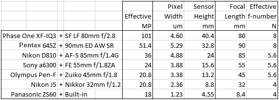
The following fits refer to the green channel of a number of interchangeable lens digital camera systems with different lenses, pixel sizes and formats – from the current Medium Format 100MP champ to the 1/2.3″ 18MP sensor size also sometimes found in the best smartphones. Here is the roster with the cameras as set up:
The series of articles starting here outlines a model of how the various physical components of a digital camera and lens can affect the ‘sharpness’ – that is the spatial resolution – of the images captured in the raw data. In this one we will pit the model against MTF curves obtained through the slanted edge method[1]from real world raw captures both with and without an anti-aliasing filter.
With a few simplifying assumptions, which include ignoring aliasing and phase, the spatial frequency response (SFR or MTF) of a photographic digital imaging system near the center can be expressed as the product of the Modulation Transfer Function of each component in it. For a current digital camera these would typically be the main ones:
This article will discuss a simple frequency domain model for an AntiAliasing (or Optical Low Pass) Filter, a hardware component sometimes found in a digital imaging system[1]. The filter typically sits just above the sensor and its objective is to block as much of the aliasing and moiré creating energy above the monochrome Nyquist spatial frequency while letting through as much as possible of the real image forming energy below that, hence the low-pass designation.
Figure 1. The blue line indicates the pass through performance of an ideal anti-aliasing filter presented with an Airy PSF (Original): pass all spatial frequencies below Nyquist (0.5 c/p) and none above that. No filter has such ideal characteristics and if it did its hard edges would result in undesirable ringing in the image.
In consumer digital cameras it is often implemented by introducing one or two birefringent plates in the sensor’s filter stack. This is how Nikon shows it for one of its DSLRs:
Figure 2. Typical Optical Low Pass Filter implementation in a current Digital Camera, courtesy of Nikon USA (yellow displacement ‘d’ added).
Having shown that our simple two dimensional MTF model is able to predict the performance of the combination of a perfect lens and square monochrome pixel with 100% Fill Factor we now turn to the effect of the sampling interval on spatial resolution according to the guiding formula:
(1)
The hats in this case mean the Fourier Transform of the relative component normalized to 1 at the origin (), that is the individual MTFs of the perfect lens PSF, the perfect square pixel and the delta grid; represents two dimensional convolution.
Sampling in the Spatial Domain
While exposed a pixel sees the scene through its aperture and accumulates energy as photons arrive. Below left is the representation of, say, the intensity that a star projects on the sensing plane, in this case resulting in an Airy pattern since we said that the lens is perfect. During exposure each pixel integrates (counts) the arriving photons, an operation that mathematically can be expressed as the convolution of the shown Airy pattern with a square, the size of effective pixel aperture, here assumed to have 100% Fill Factor. It is the convolution in the continuous spatial domain of lens PSF with pixel aperture PSF shown in Equation (2) of the first article in the series.
Sampling is then the product of an infinitesimally small Dirac delta function at the center of each pixel, the red dots below left, by the result of the convolution, producing the sampled image below right.
Figure 1. Left, 1a: A highly zoomed (3200%) image of the lens PSF, an Airy pattern, projected onto the imaging plane where the sensor sits. Pixels shown outlined in yellow. A red dot marks the sampling coordinates. Right, 1b: The sampled image zoomed at 16000%, 5x as much, because in this example each pixel’s width is 5 linear units on the side.
The next few posts will describe a linear spatial resolution model that can help a photographer better understand the main variables involved in evaluating the ‘sharpness’ of photographic equipment and related captures. I will show numerically that the combined spectral frequency response (MTF) of a perfect AAless monochrome digital camera and lens in two dimensions can be described as the magnitude of the normalized product of the Fourier Transform (FT) of the lens Point Spread Function by the FT of the pixel footprint (aperture), convolved with the FT of a rectangular grid of Dirac delta functions centered at each pixel:
With a few simplifying assumptions we will see that the effect of the lens and sensor on the spatial resolution of the continuous image on the sensing plane can be broken down into these simple components. The overall ‘sharpness’ of the captured digital image can then be estimated by combining the ‘sharpness’ of each of them.
Olympus just announced the E-M5 Mark II, an updated version of its popular micro Four Thirds E-M5 model, with an interesting new feature: its 16MegaPixel sensor, presumably similar to the one in other E-Mx bodies, has a high resolution mode where it gets shifted around by the image stabilization servos during exposure to capture, as they say in their press release
‘resolution that goes beyond full-frame DSLR cameras. 8 images are captured with 16-megapixel image information while moving the sensor by 0.5 pixel steps between each shot. The data from the 8 shots are then combined to produce a single, super-high resolution image, equivalent to the one captured with a 40-megapixel image sensor.’
A great idea that could give a welcome boost to the ‘sharpness’ of this handy system. Preliminary tests show that the E-M5 mk II 64MP High-Res mode gives some advantage in MTF50 linear spatial resolution compared to the Standard Shot 16MP mode with the captures in this post. Plus it apparently virtually eliminates the possibility of aliasing and moiré. Great stuff, Olympus.
Several sites for photographers perform spatial resolution ‘sharpness’ testing of a specific lens and digital camera set up by capturing a target. You can also measure your own equipment relatively easily to determine how sharp your hardware is. However comparing results from site to site and to your own can be difficult and/or misleading, starting from the multiplicity of units used: cycles/pixel, line pairs/mm, line widths/picture height, line pairs/image height, cycles/picture height etc.
This post will address the units involved in spatial resolution measurement using as an example readings from the popular slanted edge method, although their applicability is generic.
The following approach will work if you know the spatial frequency at which a certain MTF relative energy level (e.g. MTF50) is achieved by your camera/lens combination as set up at the time that the capture was taken.


 ), that is the individual MTFs of the perfect lens PSF, the perfect square pixel and the delta grid;
  represents two dimensional convolution.
![\[ MTF_{2D} = \left|\widehat{ PSF_{lens} }\cdot \widehat{PIX_{ap} }\right|_{pu}\ast\ast\: \delta\widehat{\delta_{pitch}} \]](https://i0.wp.com/www.strollswithmydog.com/wordpress/wp-content/ql-cache/quicklatex.com-3409f065a49bb47fd4618ed595be72fc_l3.png?resize=320%2C37&ssl=1 "Rendered by QuickLaTeX.com")