Tag Archives: deconvolution

The Nikon Z7’s Insane Sharpness

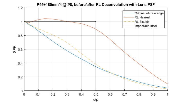
Ever since getting a Nikon Z7 MILC a few months ago I have been literally blown away by the level of sharpness it produces.   I thought that my surprise might be the result of moving up from 24 to 45.7MP, or the excellent pin-point focusing mode, or the lack of an Antialiasing filter.  Well, it turns out that there is probably more at work than that.

This weekend I pulled out the largest cutter blade I could find and set it up rough and tumble near vertically about 10 meters away  to take a peek at what the MTF curves that produce such sharp results might look like.

Continue reading The Nikon Z7’s Insane Sharpness

The Richardson-Lucy Algorithm

Deconvolution by the Richardson-Lucy algorithm is achieved by minimizing the convex loss function derived in the last article

(1)   \begin{equation*} J(O) = \sum \bigg (O**PSF - I\cdot ln(O**PSF) \bigg) \end{equation*}

with

  • J, the scalar quantity to minimize, function of ideal image O(x,y)
  • I(x,y), linear captured image intensity laid out in M rows and N columns, corrupted by Poisson noise and blurring by the PSF
  • PSF(x,y), the known two-dimensional Point Spread Function that should be deconvolved out of I
  • O(x,y), the output image resulting from deconvolution, ideally without shot noise and blurring introduced by the PSF
  • **   two-dimensional convolution
  • \cdot   element-wise product
  • ln, element-wise natural logarithm

In what follows indices x and y, from zero to M-1 and N-1 respectively, are dropped for readability.  Articles about algorithms are by definition dry so continue at your own peril.

So, given captured raw image I blurred by known function PSF, how do we find the minimum value of J yielding the deconvolved image O that we are after?

Continue reading The Richardson-Lucy Algorithm

Elements of Richardson-Lucy Deconvolution

We have seen that deconvolution by naive division in the frequency domain only works in ideal conditions not typically found in normal photographic settings, in part because of shot noise inherent in light from the scene. Half a century ago William Richardson (1972)[1] and Leon Lucy (1974)[2] independently came up with a better way to deconvolve blurring introduced by an imaging system in the presence of shot noise. Continue reading Elements of Richardson-Lucy Deconvolution

Capture Sharpening: Estimating Lens PSF

The next few articles will outline the first tiny few steps towards achieving perfect capture sharpening, that is deconvolution of an image by the Point Spread Function (PSF) of the lens used to capture it.  This is admittedly  a complex subject, fraught with a myriad ever changing variables even in a lab, let alone in the field.  But studying it can give a glimpse of the possibilities and insights into the processes involved.

I will explain the steps I followed and show the resulting images and measurements.  Jumping the gun, the blue line below represents the starting system Spatial Frequency Response (SFR)[1], the black one unattainable/undesirable perfection and the orange one the result of part of the process outlined in this series.

Figure 1. Spatial Frequency Response of the imaging system before and after Richardson-Lucy deconvolution by the PSF of the lens that captured the original image.

Continue reading Capture Sharpening: Estimating Lens PSF

Deconvolution PSF Changes with Aperture

We have  seen in the previous post how the radius for deconvolution capture sharpening by a Gaussian PSF can be estimated for a given setup in well behaved and characterized camera systems.  Some parameters like pixel aperture and AA strength should remain stable for a camera/prime lens combination as f-numbers are increased (aperture is decreased) from about f/5.6 on up – the f/stops dear to Full Frame landscape photographers.  But how should the radius for generic Gaussian deconvolution  change as the f-number increases from there? Continue reading Deconvolution PSF Changes with Aperture

What Radius to Use for Deconvolution Capture Sharpening

The following approach will work if you know the spatial frequency at which a certain MTF relative energy level (e.g. MTF50) is achieved by your camera/lens combination as set up at the time that the capture was taken.

The process by which our hardware captures images and stores them  in the raw data inevitably blurs detail information from the scene. Continue reading What Radius to Use for Deconvolution Capture Sharpening

Deconvolution vs USM Capture Sharpening

UnSharp Masking (USM) capture sharpening is somewhat equivalent to taking a black/white marker and drawing along every transition in the picture to make it stand out more – automatically.  Line thickness and darkness is chosen arbitrarily to achieve the desired effect, much like painters do. Continue reading Deconvolution vs USM Capture Sharpening