As a landscape shooter I often wonder whether old rules for DOF still apply to current small pixels and sharp lenses. I therefore roughly measured the spatial resolution performance of my Z7 with 24-70mm/4 S in the center to see whether ‘f/8 and be there’ still made sense today. The journey and the diffraction-simple-aberration aware model were described in the last few posts. The results are summarized in the Landscape Aperture-Distance charts presented here for the 24, 28 and 35mm focal lengths.
I also present the data in the form of a simplified plot to aid making the right compromises when the focusing distance is flexible. This information is valid for the Z7 and kit in the center only. It probably just as easily applies to cameras with similarly spec’d pixels and lenses. Continue reading Diffracted DOF Aperture Guides: 24-35mm→
After an exhausting two and a half hour hike you are finally resting, sitting on a rock at the foot of your destination, a tiny alpine lake, breathing in the thin air and absorbing the majestic scenery. A cool light breeze suddenly rips the surface of the water, morphing what has until now been a perfect reflection into an impressionistic interpretation of the impervious mountains in the distance.
The beautiful flowers in the foreground are so close you can touch them, the reflection in the water 10-20m away, the imposing mountains in the background a few hundred meters further out. You realize you are hungry. As you search the backpack for the two panini you prepared this morning you begin to ponder how best to capture the scene: subject, composition, Exposure, Depth of Field.
Figure 1. A typical landscape situation: a foreground a few meters away, a mid-ground a few tens and a background a few hundred meters further out. Three orders of magnitude. The focus point was on the running dog, f/16, 1/100s. Was this a good choice?
Depth of Field. Where to focus and at what f/stop? You tip your hat and just as you look up at the bluest of blue skies the number 16 starts enveloping your mind, like rays from the warm noon sun. You dial it in and as you squeeze the trigger that familiar nagging question bubbles up, as it always does in such conditions. If this were a one shot deal, was that really the best choice?
In this article we attempt to provide information to make explicit some of the trade-offs necessary in the choice of Aperture for 24mm landscapes. The result of the process is a set of guidelines. The answers are based on the previously introduced diffraction-aware model for sharpness in the center along the depth of the field – and a tripod-mounted Nikon Z7 + Nikkor 24-70mm/4 S kit lens at 24mm. Continue reading DOF and Diffraction: 24mm Guidelines→
The two-thin-lens model for precision Depth Of Field estimates described in the last two articles is almost ready to be deployed. In this one we will describe the setup that will be used to develop the scenarios that will be outlined in the next one.
The beauty of the hybrid geometrical-Fourier optics approach is that, with an estimate of the field produced at the exit pupil by an on-axis point source, we can generate the image of the resulting Point Spread Function and related Modulation Transfer Function.
Pretend that you are a photon from such a source in front of a f/2.8 lens focused at 10m with about 0.60 microns of third order spherical aberration – and you are about to smash yourself onto the ‘best focus’ observation plane of your camera. Depending on whether you leave exactly from the in-focus distance of 10 meters or slightly before/after that, the impression you would leave on the sensing plane would look as follows:
Figure 1. PSF of a lens with about 0.6um of third order spherical aberration focused on 10m.
The width of the square above is 30 microns (um), which corresponds to the diameter of the Circle of Confusion used for old-fashioned geometrical DOF calculations with full frame cameras. The first ring of the in-focus PSF at 10.0m has a diameter of about 2.44 = 3.65 microns. That’s about the size of the estimated effective square pixel aperture of the Nikon Z7 camera that we are using in these tests. Continue reading DOF and Diffraction: Setup→
This investigation of the effect of diffraction on Depth of Field is based on a two-thin-lens model, as suggested by Alan Robinson[1]. We chose this model because it allows us to associate geometrical optics with one lens and Fourier optics with the other, thus simplifying the underlying math and our understanding.
In the last article we discussed how the front element of the model could present at the rear element the wavefront resulting from an on-axis source as a function of distance from the lens. We accomplished this by using simple geometry in complex notation. In this one we will take the relative wavefront present at the exit pupil and project it onto the sensing plane, taking diffraction into account numerically. We already know how to do it since we dealt with this subject in the recent past.
Figure 1. Where is the plane with the Circle of Least Confusion? Through Focus Line Spread Function Image of a lens at f/2.8 with the indicated third order spherical aberration coefficient, and relative measures of ‘sharpness’ MTF50 and Acutance curves. Acutance is scaled to the same peak as MTF50 for ease of comparison and refers to my typical pixel peeping conditions: 100% zoom, 16″ away from my 24″ monitor.
In this and the following articles we shall explore the effects of diffraction on Depth of Field through a two-lens model that separates geometrical and Fourier optics in a way that keeps the math simple, though via complex notation. In the process we will gain a better understanding of how lenses work.
The results of the model are consistent with what can be obtained via classic DOF calculators online but should be more precise in critical situations, like macro photography. I am not a macro photographer so I would be interested in validation of the results of the explained method by someone who is.
Figure 1. Simple two-thin-lens model for DOF calculations in complex notation. Adapted under licence.
Goodman, in his excellent Introduction to Fourier Optics[1], describes how an image is formed on a camera sensing plane starting from first principles, that is electromagnetic propagation according to Maxwell’s wave equation. If you want the play by play account I highly recommend his math intensive book. But for the budding photographer it is sufficient to know what happens at the Exit Pupil of the lens because after that the transformations to Point Spread and Modulation Transfer Functions are straightforward, as we will show in this article.
The following diagram exemplifies the last few millimeters of the journey that light from the scene has to travel in order to be absorbed by a camera’s sensing medium. Light from the scene in the form of field arrives at the front of the lens. It goes through the lens being partly blocked and distorted by it as it arrives at its virtual back end, the Exit Pupil, we’ll call this blocking/distorting function . Other than in very simple cases, the Exit Pupil does not necessarily coincide with a specific physical element or Principal surface.[iv] It is a convenient mathematical construct which condenses all of the light transforming properties of a lens into a single plane.
The complex light field at the Exit Pupil’s two dimensional plane is then as shown below (not to scale, the product of the two arrays is element-by-element):
Figure 1. Simplified schematic diagram of the space between the exit pupil of a camera lens and its sensing plane. The space is assumed to be filled with air.
This post will continue looking at the spatial frequency response measured by MTF Mapper off slanted edges in DPReview.com raw captures and relative fits by the ‘sharpness’ model discussed in the last few articles. The model takes the physical parameters of the digital camera and lens as inputs and produces theoretical directional system MTF curves comparable to measured data. As we will see the model seems to be able to simulate these systems well – at least within this limited set of parameters.
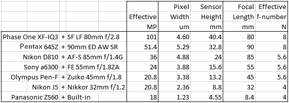
The following fits refer to the green channel of a number of interchangeable lens digital camera systems with different lenses, pixel sizes and formats – from the current Medium Format 100MP champ to the 1/2.3″ 18MP sensor size also sometimes found in the best smartphones. Here is the roster with the cameras as set up:
The series of articles starting here outlines a model of how the various physical components of a digital camera and lens can affect the ‘sharpness’ – that is the spatial resolution – of the images captured in the raw data. In this one we will pit the model against MTF curves obtained through the slanted edge method[1]from real world raw captures both with and without an anti-aliasing filter.
With a few simplifying assumptions, which include ignoring aliasing and phase, the spatial frequency response (SFR or MTF) of a photographic digital imaging system near the center can be expressed as the product of the Modulation Transfer Function of each component in it. For a current digital camera these would typically be the main ones:
We now know how to calculate the two dimensional Modulation Transfer Function of a perfect lens affected by diffraction, defocus and third order Spherical Aberration – under monochromatic light at the given wavelength and f-number. In digital photography however we almost never deal with light of a single wavelength. So what effect does an illuminant with a wide spectral power distribution, going through the color filter of a typical digital camera CFA before the sensor have on the spatial frequency responses discussed thus far?
This article is about specifying the units of the Discrete Fourier Transform of an image and the various ways that they can be expressed. This apparently simple task can be fiendishly unintuitive.
The image we will use as an example is the familiar Airy Disk from the last few posts, at f/16 with light of mean 530nm wavelength. Zoomed in to the left in Figure 1; and as it looks in its 1024×1024 sample image to the right:
Figure 1. Airy disc image I(x,y). Left, 1a, 3D representation, zoomed in. Right, 1b, as it would appear on the sensing plane (yes, the rings are there but you need to squint to see them).
Now that we know from the introductory article that the spatial frequency response of a typical perfect digital camera and lens (its Modulation Transfer Function) can be modeled simply as the product of the Fourier Transform of the Point Spread Function of the lens and pixel aperture, convolved with a Dirac delta grid at cycles-per-pixel pitch spacing
The next few posts will describe a linear spatial resolution model that can help a photographer better understand the main variables involved in evaluating the ‘sharpness’ of photographic equipment and related captures. I will show numerically that the combined spectral frequency response (MTF) of a perfect AAless monochrome digital camera and lens in two dimensions can be described as the magnitude of the normalized product of the Fourier Transform (FT) of the lens Point Spread Function by the FT of the pixel footprint (aperture), convolved with the FT of a rectangular grid of Dirac delta functions centered at each pixel:
With a few simplifying assumptions we will see that the effect of the lens and sensor on the spatial resolution of the continuous image on the sensing plane can be broken down into these simple components. The overall ‘sharpness’ of the captured digital image can then be estimated by combining the ‘sharpness’ of each of them.
Equivalence – as we’ve discussed one of the fairest ways to compare the performance of two cameras of different physical formats, characteristics and specifications – essentially boils down to two simple realizations for digital photographers:
metrics need to be expressed in units of picture height (or diagonal where the aspect ratio is significantly different) in order to easily compare performance with images displayed at the same size; and
focal length changes proportionally to sensor size in order to capture identical scene content on a given sensor, all other things being equal.
The first realization should be intuitive (see next post). The second one is the subject of this post: I will deal with it through a couple of geometrical diagrams.


 = 3.65 microns. That’s about the size of the estimated effective square pixel aperture of the Nikon Z7 camera that we are using in these tests.

 arrives at the front of the lens. It goes through the lens being partly blocked and distorted by it as it arrives at its virtual back end, the Exit Pupil, we’ll call this blocking/distorting function
  . Other than in very simple cases, the Exit Pupil does not necessarily coincide with a specific physical element or Principal surface.
 plane is then
  as shown below (not to scale, the product of the two arrays is element-by-element):


 here indicating normalization to one at the origin). I used Matlab to generate the examples below but you can easily do the same with a spreadsheet.
 ![\[ MTF_{2D} = \left|\widehat{ PSF_{lens} }\cdot \widehat{PIX_{ap} }\right|_{pu}\ast\ast\: \delta\widehat{\delta_{pitch}} \]](https://i0.wp.com/www.strollswithmydog.com/wordpress/wp-content/ql-cache/quicklatex.com-3409f065a49bb47fd4618ed595be72fc_l3.png?resize=320%2C37&ssl=1 "Rendered by QuickLaTeX.com")