Ever since getting a Nikon Z7 MILC a few months ago I have been literally blown away by the level of sharpness it produces. I thought that my surprise might be the result of moving up from 24 to 45.7MP, or the excellent pin-point focusing mode, or the lack of an Antialiasing filter. Well, it turns out that there is probably more at work than that.
This weekend I pulled out the largest cutter blade I could find and set it up rough and tumble near vertically about 10 meters away to take a peek at what the MTF curves that produce such sharp results might look like.
Canon recently introduced its EOS-1D X Mark III Digital Single-Lens Reflex [Edit: and now also possibly the R5 Mirrorless ILC] touting a new and improved Anti-Aliasing filter, which they call a High-Res Gaussian Distribution LPF, claiming that
“This not only helps to suppress moiré and color distortion, but also improves resolution.”
Figure 1. Artist’s rendition of new High-res Low Pass Filter, courtesy of Canon USA
In this article we will try to dissect the marketing speak and understand a bit better the theoretical implications of the new AA. For the abridged version, jump to the Conclusions at the bottom. In a picture:
This post will continue looking at the spatial frequency response measured by MTF Mapper off slanted edges in DPReview.com raw captures and relative fits by the ‘sharpness’ model discussed in the last few articles. The model takes the physical parameters of the digital camera and lens as inputs and produces theoretical directional system MTF curves comparable to measured data. As we will see the model seems to be able to simulate these systems well – at least within this limited set of parameters.
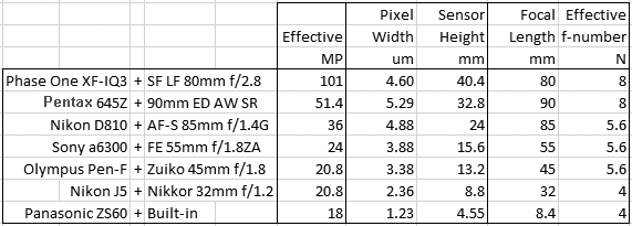
The following fits refer to the green channel of a number of interchangeable lens digital camera systems with different lenses, pixel sizes and formats – from the current Medium Format 100MP champ to the 1/2.3″ 18MP sensor size also sometimes found in the best smartphones. Here is the roster with the cameras as set up:
Having shown that our simple two dimensional MTF model is able to predict the performance of the combination of a perfect lens and square monochrome pixel with 100% Fill Factor we now turn to the effect of the sampling interval on spatial resolution according to the guiding formula:
(1)
The hats in this case mean the Fourier Transform of the relative component normalized to 1 at the origin (), that is the individual MTFs of the perfect lens PSF, the perfect square pixel and the delta grid; represents two dimensional convolution.
Sampling in the Spatial Domain
While exposed a pixel sees the scene through its aperture and accumulates energy as photons arrive. Below left is the representation of, say, the intensity that a star projects on the sensing plane, in this case resulting in an Airy pattern since we said that the lens is perfect. During exposure each pixel integrates (counts) the arriving photons, an operation that mathematically can be expressed as the convolution of the shown Airy pattern with a square, the size of effective pixel aperture, here assumed to have 100% Fill Factor. It is the convolution in the continuous spatial domain of lens PSF with pixel aperture PSF shown in Equation (2) of the first article in the series.
Sampling is then the product of an infinitesimally small Dirac delta function at the center of each pixel, the red dots below left, by the result of the convolution, producing the sampled image below right.
Figure 1. Left, 1a: A highly zoomed (3200%) image of the lens PSF, an Airy pattern, projected onto the imaging plane where the sensor sits. Pixels shown outlined in yellow. A red dot marks the sampling coordinates. Right, 1b: The sampled image zoomed at 16000%, 5x as much, because in this example each pixel’s width is 5 linear units on the side.
Olympus just announced the E-M5 Mark II, an updated version of its popular micro Four Thirds E-M5 model, with an interesting new feature: its 16MegaPixel sensor, presumably similar to the one in other E-Mx bodies, has a high resolution mode where it gets shifted around by the image stabilization servos during exposure to capture, as they say in their press release
‘resolution that goes beyond full-frame DSLR cameras. 8 images are captured with 16-megapixel image information while moving the sensor by 0.5 pixel steps between each shot. The data from the 8 shots are then combined to produce a single, super-high resolution image, equivalent to the one captured with a 40-megapixel image sensor.’
A great idea that could give a welcome boost to the ‘sharpness’ of this handy system. Preliminary tests show that the E-M5 mk II 64MP High-Res mode gives some advantage in MTF50 linear spatial resolution compared to the Standard Shot 16MP mode with the captures in this post. Plus it apparently virtually eliminates the possibility of aliasing and moiré. Great stuff, Olympus.
My preferred method for measuring the spatial resolution performance of photographic equipment these days is the slanted edge method. It requires a minimum amount of additional effort compared to capturing and simply eye-balling a pinch, Siemens or other chart but it gives immensely more, useful, accurate, quantitative information in the language and units that have been used to characterize optical systems for over a century: it produces a good approximation to the Modulation Transfer Function of the two dimensional camera/lens system impulse response – at the location of the edge in the direction perpendicular to it.
Much of what there is to know about an imaging system’s spatial resolution performance can be deduced by analyzing its MTF curve, which represents the system’s ability to capture increasingly fine detail from the scene, starting from perceptually relevant metrics like MTF50, discussed a while back. In fact the area under the curve weighted by some approximation of the Contrast Sensitivity Function of the Human Visual System is the basis for many other, better accepted single figure ‘sharpness‘ metrics with names like Subjective Quality Factor (SQF), Square Root Integral (SQRI), CMT Acutance, etc. And all this simply from capturing the image of a slanted edge, which one can actually and somewhat easily do at home, as presented in the next article.


 ), that is the individual MTFs of the perfect lens PSF, the perfect square pixel and the delta grid;
  represents two dimensional convolution.