As a landscape shooter I often wonder whether old rules for DOF still apply to current small pixels and sharp lenses. I therefore roughly measured the spatial resolution performance of my Z7 with 24-70mm/4 S in the center to see whether ‘f/8 and be there’ still made sense today. The journey and the diffraction-simple-aberration aware model were described in the last few posts. The results are summarized in the Landscape Aperture-Distance charts presented here for the 24, 28 and 35mm focal lengths.
I also present the data in the form of a simplified plot to aid making the right compromises when the focusing distance is flexible. This information is valid for the Z7 and kit in the center only. It probably just as easily applies to cameras with similarly spec’d pixels and lenses. Continue reading Diffracted DOF Aperture Guides: 24-35mm→
After an exhausting two and a half hour hike you are finally resting, sitting on a rock at the foot of your destination, a tiny alpine lake, breathing in the thin air and absorbing the majestic scenery. A cool light breeze suddenly rips the surface of the water, morphing what has until now been a perfect reflection into an impressionistic interpretation of the impervious mountains in the distance.
The beautiful flowers in the foreground are so close you can touch them, the reflection in the water 10-20m away, the imposing mountains in the background a few hundred meters further out. You realize you are hungry. As you search the backpack for the two panini you prepared this morning you begin to ponder how best to capture the scene: subject, composition, Exposure, Depth of Field.
Figure 1. A typical landscape situation: a foreground a few meters away, a mid-ground a few tens and a background a few hundred meters further out. Three orders of magnitude. The focus point was on the running dog, f/16, 1/100s. Was this a good choice?
Depth of Field. Where to focus and at what f/stop? You tip your hat and just as you look up at the bluest of blue skies the number 16 starts enveloping your mind, like rays from the warm noon sun. You dial it in and as you squeeze the trigger that familiar nagging question bubbles up, as it always does in such conditions. If this were a one shot deal, was that really the best choice?
In this article we attempt to provide information to make explicit some of the trade-offs necessary in the choice of Aperture for 24mm landscapes. The result of the process is a set of guidelines. The answers are based on the previously introduced diffraction-aware model for sharpness in the center along the depth of the field – and a tripod-mounted Nikon Z7 + Nikkor 24-70mm/4 S kit lens at 24mm. Continue reading DOF and Diffraction: 24mm Guidelines→
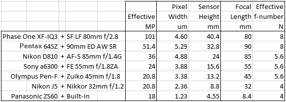
This post will continue looking at the spatial frequency response measured by MTF Mapper off slanted edges in DPReview.com raw captures and relative fits by the ‘sharpness’ model discussed in the last few articles. The model takes the physical parameters of the digital camera and lens as inputs and produces theoretical directional system MTF curves comparable to measured data. As we will see the model seems to be able to simulate these systems well – at least within this limited set of parameters.
The following fits refer to the green channel of a number of interchangeable lens digital camera systems with different lenses, pixel sizes and formats – from the current Medium Format 100MP champ to the 1/2.3″ 18MP sensor size also sometimes found in the best smartphones. Here is the roster with the cameras as set up:
Now that we know from the introductory article that the spatial frequency response of a typical perfect digital camera and lens (its Modulation Transfer Function) can be modeled simply as the product of the Fourier Transform of the Point Spread Function of the lens and pixel aperture, convolved with a Dirac delta grid at cycles-per-pixel pitch spacing
While perusing Jim Kasson’s excellent Longitudinal Chromatic Aberration tests[1] I was impressed by the quantity and quality of the information the resulting data provides. Longitudinal, or Axial, CA is a form of defocus and as such it cannot be effectively corrected during raw conversion, so having a lens well compensated for it will provide a real and tangible improvement in the sharpness of final images. How much of an improvement?
In this and the previous article I present my thoughts on how MTF50 results obtained from raw data of the four Bayer CFA channels – off a uniformly illuminated neutral target captured with a typical digital camera through the slanted edge method – can be combined to provide a meaningful composite MTF50 for the imaging system as a whole1. Corrections, suggestions and challenges are welcome. Continue reading COMBINING BAYER CFA MTF Curves – II→
In this and the following article I will discuss my thoughts on how MTF50 results obtained from raw data of the four Bayer CFA color channels off a neutral target captured with a typical camera through the slanted edge method can be combined to provide a meaningful composite MTF50 for the imaging system as a whole. The perimeter of the discussion are neutral slanted edge measurements of Bayer CFA raw data for linear spatial resolution (‘sharpness’) photographic hardware evaluations. Corrections, suggestions and challenges are welcome. Continue reading Combining Bayer CFA Modulation Transfer Functions – I→
Over the last couple of years I’ve been using Frans van den Bergh‘s excellent open source MTF Mapper to measure the Modulation Transfer Function of imaging systems off a slanted edge target, as you may have seen in these pages. As long as one understands how to get the most out of it I find it a solid product that gives reliable results, with MTF50 typically well within 2% of actual in less than ideal real-world situations (see below). I had little to compare it to other than to tests published by gear testing sites: they apparently mostly use a commercial package called Imatest for their slanted edge readings – and it seemed to correlate well with those.
Then recently Jim Kasson pointed out sfrmat3, the matlab program written by Peter Burns who is a slanted edge method expert who worked at Kodak and was a member of the committee responsible for ISO12233, the resolution and spatial frequency response standard for photography. sfrmat3 is considered to be a solid implementation of the standard and many, including Imatest, benchmark against it – so I was curious to see how MTF Mapper 0.4.1.6 would compare. It did well.
Olympus just announced the E-M5 Mark II, an updated version of its popular micro Four Thirds E-M5 model, with an interesting new feature: its 16MegaPixel sensor, presumably similar to the one in other E-Mx bodies, has a high resolution mode where it gets shifted around by the image stabilization servos during exposure to capture, as they say in their press release
‘resolution that goes beyond full-frame DSLR cameras. 8 images are captured with 16-megapixel image information while moving the sensor by 0.5 pixel steps between each shot. The data from the 8 shots are then combined to produce a single, super-high resolution image, equivalent to the one captured with a 40-megapixel image sensor.’
A great idea that could give a welcome boost to the ‘sharpness’ of this handy system. Preliminary tests show that the E-M5 mk II 64MP High-Res mode gives some advantage in MTF50 linear spatial resolution compared to the Standard Shot 16MP mode with the captures in this post. Plus it apparently virtually eliminates the possibility of aliasing and moiré. Great stuff, Olympus.
So, is it true that a Four Thirds lens needs to be about twice as ‘sharp’ as its Full Frame counterpart in order to be able to display an image of spatial resolution equivalent to the larger format’s?
It is, because of the simple geometry I will describe in this article. In fact with a few provisos one can generalize and say that lenses from any smaller format need to be ‘sharper’ by the ratio of their sensor diagonals in order to produce the same linear resolution on same-sized final images.
This is one of the reasons why Ansel Adams shot 4×5 and 8×10 – and I would too, were it not for logistical and pecuniary concerns.
Several sites for photographers perform spatial resolution ‘sharpness’ testing of a specific lens and digital camera set up by capturing a target. You can also measure your own equipment relatively easily to determine how sharp your hardware is. However comparing results from site to site and to your own can be difficult and/or misleading, starting from the multiplicity of units used: cycles/pixel, line pairs/mm, line widths/picture height, line pairs/image height, cycles/picture height etc.
This post will address the units involved in spatial resolution measurement using as an example readings from the popular slanted edge method, although their applicability is generic.
You have obtained a raw file containing the image of a slanted edge captured with good technique. How do you get the Modulation Transfer Function of the camera and lens combination that took it? Download and feast your eyes on open source MTF Mapper version 0.4.16 by Frans van den Bergh.
[Edit 2023: MTF Mapper has kept improving over the years, making it in my opinion the most accurate slanted edge measuring tool available today, used in applications that range from photography to machine vision to the Mars Rover. Did I mention that it is open source?
It now sports a Graphical User Interface which can load raw files and allow the arbitrary selection of individual edges by simply pointing and clicking, making this post largely redundant. The procedure outlined below will still work but there are easier ways to accomplish the same task today: just “File/Open single edge image” raw files from the GUI after having inserted “–bayer green” in the additional string field. Thanks Frans.]
The first thing we are going to do is crop the edges and package them into a TIFF file format so that MTF Mapper has an easier time reading them. Let’s use as an example a Nikon D810+85mm:1.8G ISO 64 studio raw capture by DPReview so that you can follow along if you wish. Continue reading How to Get MTF Performance Curves for Your Camera and Lens→
My preferred method for measuring the spatial resolution performance of photographic equipment these days is the slanted edge method. It requires a minimum amount of additional effort compared to capturing and simply eye-balling a pinch, Siemens or other chart but it gives immensely more, useful, accurate, quantitative information in the language and units that have been used to characterize optical systems for over a century: it produces a good approximation to the Modulation Transfer Function of the two dimensional camera/lens system impulse response – at the location of the edge in the direction perpendicular to it.
Much of what there is to know about an imaging system’s spatial resolution performance can be deduced by analyzing its MTF curve, which represents the system’s ability to capture increasingly fine detail from the scene, starting from perceptually relevant metrics like MTF50, discussed a while back. In fact the area under the curve weighted by some approximation of the Contrast Sensitivity Function of the Human Visual System is the basis for many other, better accepted single figure ‘sharpness‘ metrics with names like Subjective Quality Factor (SQF), Square Root Integral (SQRI), CMT Acutance, etc. And all this simply from capturing the image of a slanted edge, which one can actually and somewhat easily do at home, as presented in the next article.
Why Raw? The question is whether one is interested in measuring the objective, quantitative spatial resolution capabilities of the hardware or whether instead one would prefer to measure the arbitrary, qualitatively perceived sharpening prowess of (in-camera or in-computer) processing software as it turns the capture into a pleasing final image. Either is of course fine.
My take on this is that the better the IQ captured the better the final image will be after post processing. In other words I am typically more interested in measuring the spatial resolution information produced by the hardware comfortable in the knowledge that if I’ve got good quality data to start with its appearance will only be improved in post by the judicious use of software. By IQ here I mean objective, reproducible, measurable physical quantities representing the quality of the information captured by the hardware, ideally in scientific units.
You want to measure how sharp your camera/lens combination is to make sure it lives up to its specs. Or perhaps you’d like to compare how well one lens captures spatial resolution compared to another you own. Or perhaps again you are in the market for new equipment and would like to know what could be expected from the shortlist. Or an old faithful is not looking right and you’d like to check it out. So you decide to do some testing. Where to start?
In the next four articles I will walk you through my methodology based on captures of slanted edge targets:
Is MTF50 a good proxy for perceived sharpness? In this article and those that follow MTF50 indicates the spatial frequency at which the Modulation Transfer Function of an imaging system is half (50%) of what it would be if the system did not degrade detail in the image painted by incoming light.
It makes intuitive sense that the spatial frequencies that are most closely related to our perception of sharpness vary with the size and viewing distance of the displayed image.
For instance if an image captured by a Full Frame camera is viewed at ‘standard’ distance (that is a distance equal to its diagonal), it turns out that the portion of the MTF curve most representative of perceived sharpness appears to be around MTF90. On the other hand, when pixel peeping, the spatial frequencies around MTF50 look to be a decent, simple to calculate indicator of it with a current imaging system in good working conditions. Continue reading MTF50 and Perceived Sharpness→
The following approach will work if you know the spatial frequency at which a certain MTF relative energy level (e.g. MTF50) is achieved by your camera/lens combination as set up at the time that the capture was taken.


 here indicating normalization to one at the origin). I used Matlab to generate the examples below but you can easily do the same with a spreadsheet.