As a landscape shooter I often wonder whether old rules for DOF still apply to current small pixels and sharp lenses. I therefore roughly measured the spatial resolution performance of my Z7 with 24-70mm/4 S in the center to see whether ‘f/8 and be there’ still made sense today. The journey and the diffraction-simple-aberration aware model were described in the last few posts. The results are summarized in the Landscape Aperture-Distance charts presented here for the 24, 28 and 35mm focal lengths.
I also present the data in the form of a simplified plot to aid making the right compromises when the focusing distance is flexible. This information is valid for the Z7 and kit in the center only. It probably just as easily applies to cameras with similarly spec’d pixels and lenses. Continue reading Diffracted DOF Aperture Guides: 24-35mm→
After an exhausting two and a half hour hike you are finally resting, sitting on a rock at the foot of your destination, a tiny alpine lake, breathing in the thin air and absorbing the majestic scenery. A cool light breeze suddenly rips the surface of the water, morphing what has until now been a perfect reflection into an impressionistic interpretation of the impervious mountains in the distance.
The beautiful flowers in the foreground are so close you can touch them, the reflection in the water 10-20m away, the imposing mountains in the background a few hundred meters further out. You realize you are hungry. As you search the backpack for the two panini you prepared this morning you begin to ponder how best to capture the scene: subject, composition, Exposure, Depth of Field.
Figure 1. A typical landscape situation: a foreground a few meters away, a mid-ground a few tens and a background a few hundred meters further out. Three orders of magnitude. The focus point was on the running dog, f/16, 1/100s. Was this a good choice?
Depth of Field. Where to focus and at what f/stop? You tip your hat and just as you look up at the bluest of blue skies the number 16 starts enveloping your mind, like rays from the warm noon sun. You dial it in and as you squeeze the trigger that familiar nagging question bubbles up, as it always does in such conditions. If this were a one shot deal, was that really the best choice?
In this article we attempt to provide information to make explicit some of the trade-offs necessary in the choice of Aperture for 24mm landscapes. The result of the process is a set of guidelines. The answers are based on the previously introduced diffraction-aware model for sharpness in the center along the depth of the field – and a tripod-mounted Nikon Z7 + Nikkor 24-70mm/4 S kit lens at 24mm. Continue reading DOF and Diffraction: 24mm Guidelines→
The two-thin-lens model for precision Depth Of Field estimates described in the last two articles is almost ready to be deployed. In this one we will describe the setup that will be used to develop the scenarios that will be outlined in the next one.
The beauty of the hybrid geometrical-Fourier optics approach is that, with an estimate of the field produced at the exit pupil by an on-axis point source, we can generate the image of the resulting Point Spread Function and related Modulation Transfer Function.
Pretend that you are a photon from such a source in front of a f/2.8 lens focused at 10m with about 0.60 microns of third order spherical aberration – and you are about to smash yourself onto the ‘best focus’ observation plane of your camera. Depending on whether you leave exactly from the in-focus distance of 10 meters or slightly before/after that, the impression you would leave on the sensing plane would look as follows:
Figure 1. PSF of a lens with about 0.6um of third order spherical aberration focused on 10m.
The width of the square above is 30 microns (um), which corresponds to the diameter of the Circle of Confusion used for old-fashioned geometrical DOF calculations with full frame cameras. The first ring of the in-focus PSF at 10.0m has a diameter of about 2.44 = 3.65 microns. That’s about the size of the estimated effective square pixel aperture of the Nikon Z7 camera that we are using in these tests. Continue reading DOF and Diffraction: Setup→
This investigation of the effect of diffraction on Depth of Field is based on a two-thin-lens model, as suggested by Alan Robinson[1]. We chose this model because it allows us to associate geometrical optics with one lens and Fourier optics with the other, thus simplifying the underlying math and our understanding.
In the last article we discussed how the front element of the model could present at the rear element the wavefront resulting from an on-axis source as a function of distance from the lens. We accomplished this by using simple geometry in complex notation. In this one we will take the relative wavefront present at the exit pupil and project it onto the sensing plane, taking diffraction into account numerically. We already know how to do it since we dealt with this subject in the recent past.
Figure 1. Where is the plane with the Circle of Least Confusion? Through Focus Line Spread Function Image of a lens at f/2.8 with the indicated third order spherical aberration coefficient, and relative measures of ‘sharpness’ MTF50 and Acutance curves. Acutance is scaled to the same peak as MTF50 for ease of comparison and refers to my typical pixel peeping conditions: 100% zoom, 16″ away from my 24″ monitor.
In this and the following articles we shall explore the effects of diffraction on Depth of Field through a two-lens model that separates geometrical and Fourier optics in a way that keeps the math simple, though via complex notation. In the process we will gain a better understanding of how lenses work.
The results of the model are consistent with what can be obtained via classic DOF calculators online but should be more precise in critical situations, like macro photography. I am not a macro photographer so I would be interested in validation of the results of the explained method by someone who is.
Figure 1. Simple two-thin-lens model for DOF calculations in complex notation. Adapted under licence.
Ever since getting a Nikon Z7 MILC a few months ago I have been literally blown away by the level of sharpness it produces. I thought that my surprise might be the result of moving up from 24 to 45.7MP, or the excellent pin-point focusing mode, or the lack of an Antialiasing filter. Well, it turns out that there is probably more at work than that.
This weekend I pulled out the largest cutter blade I could find and set it up rough and tumble near vertically about 10 meters away to take a peek at what the MTF curves that produce such sharp results might look like.
Canon recently introduced its EOS-1D X Mark III Digital Single-Lens Reflex [Edit: and now also possibly the R5 Mirrorless ILC] touting a new and improved Anti-Aliasing filter, which they call a High-Res Gaussian Distribution LPF, claiming that
“This not only helps to suppress moiré and color distortion, but also improves resolution.”
Figure 1. Artist’s rendition of new High-res Low Pass Filter, courtesy of Canon USA
In this article we will try to dissect the marketing speak and understand a bit better the theoretical implications of the new AA. For the abridged version, jump to the Conclusions at the bottom. In a picture:
We have seen that deconvolution by naive division in the frequency domain only works in ideal conditions not typically found in normal photographic settings, in part because of shot noise inherent in light from the scene. Half a century ago William Richardson (1972)[1] and Leon Lucy (1974)[2] independently came up with a better way to deconvolve blurring introduced by an imaging system in the presence of shot noise. Continue reading Elements of Richardson-Lucy Deconvolution→
The next few articles will outline the first tiny few steps towards achieving perfect capture sharpening, that is deconvolution of an image by the Point Spread Function (PSF) of the lens used to capture it. This is admittedly a complex subject, fraught with a myriad ever changing variables even in a lab, let alone in the field. But studying it can give a glimpse of the possibilities and insights into the processes involved.
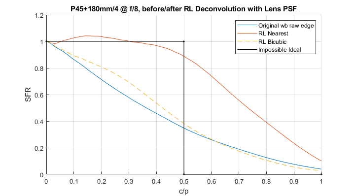
I will explain the steps I followed and show the resulting images and measurements. Jumping the gun, the blue line below represents the starting system Spatial Frequency Response (SFR)[1], the black one unattainable/undesirable perfection and the orange one the result of part of the process outlined in this series.
Figure 1. Spatial Frequency Response of the imaging system before and after Richardson-Lucy deconvolution by the PSF of the lens that captured the original image.
In this article we shall find that the effect of a Bayer CFA on the spatial frequencies and hence the ‘sharpness’ information captured by a sensor compared to those from the corresponding monochrome version can go from (almost) nothing to halving the potentially unaliased range – based on the chrominance content of the image and the direction in which the spatial frequencies are being stressed. Continue reading Bayer CFA Effect on Sharpness→
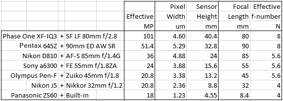
This post will continue looking at the spatial frequency response measured by MTF Mapper off slanted edges in DPReview.com raw captures and relative fits by the ‘sharpness’ model discussed in the last few articles. The model takes the physical parameters of the digital camera and lens as inputs and produces theoretical directional system MTF curves comparable to measured data. As we will see the model seems to be able to simulate these systems well – at least within this limited set of parameters.
The following fits refer to the green channel of a number of interchangeable lens digital camera systems with different lenses, pixel sizes and formats – from the current Medium Format 100MP champ to the 1/2.3″ 18MP sensor size also sometimes found in the best smartphones. Here is the roster with the cameras as set up:
The series of articles starting here outlines a model of how the various physical components of a digital camera and lens can affect the ‘sharpness’ – that is the spatial resolution – of the images captured in the raw data. In this one we will pit the model against MTF curves obtained through the slanted edge method[1]from real world raw captures both with and without an anti-aliasing filter.
With a few simplifying assumptions, which include ignoring aliasing and phase, the spatial frequency response (SFR or MTF) of a photographic digital imaging system near the center can be expressed as the product of the Modulation Transfer Function of each component in it. For a current digital camera these would typically be the main ones:
We now know how to calculate the two dimensional Modulation Transfer Function of a perfect lens affected by diffraction, defocus and third order Spherical Aberration – under monochromatic light at the given wavelength and f-number. In digital photography however we almost never deal with light of a single wavelength. So what effect does an illuminant with a wide spectral power distribution, going through the color filter of a typical digital camera CFA before the sensor have on the spatial frequency responses discussed thus far?
Spherical Aberration (SA) is one key component missing from our MTF toolkit for modeling an ideal imaging system’s ‘sharpness’ in the center of the field of view in the frequency domain. In this article formulas will be presented to compute the two dimensional Point Spread and Modulation Transfer Functions of the combination of diffraction, defocus and third order Spherical Aberration for an otherwise perfect lens with a circular aperture.
Spherical Aberrations result because most photographic lenses are designed with quasi spherical surfaces that do not necessarily behave ideally in all situations. For instance, they may focus light on systematically different planes depending on whether the respective ray goes through the exit pupil closer or farther from the optical axis, as shown below:
Figure 1. Top: an ideal spherical lens focuses all rays on the same focal point. Bottom: a practical lens with Spherical Aberration focuses rays that go through the exit pupil based on their radial distance from the optical axis. Image courtesy Andrei Stroe.
This article will discuss a simple frequency domain model for an AntiAliasing (or Optical Low Pass) Filter, a hardware component sometimes found in a digital imaging system[1]. The filter typically sits just above the sensor and its objective is to block as much of the aliasing and moiré creating energy above the monochrome Nyquist spatial frequency while letting through as much as possible of the real image forming energy below that, hence the low-pass designation.
Figure 1. The blue line indicates the pass through performance of an ideal anti-aliasing filter presented with an Airy PSF (Original): pass all spatial frequencies below Nyquist (0.5 c/p) and none above that. No filter has such ideal characteristics and if it did its hard edges would result in undesirable ringing in the image.
In consumer digital cameras it is often implemented by introducing one or two birefringent plates in the sensor’s filter stack. This is how Nikon shows it for one of its DSLRs:
Figure 2. Typical Optical Low Pass Filter implementation in a current Digital Camera, courtesy of Nikon USA (yellow displacement ‘d’ added).
Having shown that our simple two dimensional MTF model is able to predict the performance of the combination of a perfect lens and square monochrome pixel with 100% Fill Factor we now turn to the effect of the sampling interval on spatial resolution according to the guiding formula:
(1)
The hats in this case mean the Fourier Transform of the relative component normalized to 1 at the origin (), that is the individual MTFs of the perfect lens PSF, the perfect square pixel and the delta grid; represents two dimensional convolution.
Sampling in the Spatial Domain
While exposed a pixel sees the scene through its aperture and accumulates energy as photons arrive. Below left is the representation of, say, the intensity that a star projects on the sensing plane, in this case resulting in an Airy pattern since we said that the lens is perfect. During exposure each pixel integrates (counts) the arriving photons, an operation that mathematically can be expressed as the convolution of the shown Airy pattern with a square, the size of effective pixel aperture, here assumed to have 100% Fill Factor. It is the convolution in the continuous spatial domain of lens PSF with pixel aperture PSF shown in Equation (2) of the first article in the series.
Sampling is then the product of an infinitesimally small Dirac delta function at the center of each pixel, the red dots below left, by the result of the convolution, producing the sampled image below right.
Figure 1. Left, 1a: A highly zoomed (3200%) image of the lens PSF, an Airy pattern, projected onto the imaging plane where the sensor sits. Pixels shown outlined in yellow. A red dot marks the sampling coordinates. Right, 1b: The sampled image zoomed at 16000%, 5x as much, because in this example each pixel’s width is 5 linear units on the side.
Now that we know from the introductory article that the spatial frequency response of a typical perfect digital camera and lens (its Modulation Transfer Function) can be modeled simply as the product of the Fourier Transform of the Point Spread Function of the lens and pixel aperture, convolved with a Dirac delta grid at cycles-per-pixel pitch spacing
The next few posts will describe a linear spatial resolution model that can help a photographer better understand the main variables involved in evaluating the ‘sharpness’ of photographic equipment and related captures. I will show numerically that the combined spectral frequency response (MTF) of a perfect AAless monochrome digital camera and lens in two dimensions can be described as the magnitude of the normalized product of the Fourier Transform (FT) of the lens Point Spread Function by the FT of the pixel footprint (aperture), convolved with the FT of a rectangular grid of Dirac delta functions centered at each pixel:
With a few simplifying assumptions we will see that the effect of the lens and sensor on the spatial resolution of the continuous image on the sensing plane can be broken down into these simple components. The overall ‘sharpness’ of the captured digital image can then be estimated by combining the ‘sharpness’ of each of them.
While perusing Jim Kasson’s excellent Longitudinal Chromatic Aberration tests[1] I was impressed by the quantity and quality of the information the resulting data provides. Longitudinal, or Axial, CA is a form of defocus and as such it cannot be effectively corrected during raw conversion, so having a lens well compensated for it will provide a real and tangible improvement in the sharpness of final images. How much of an improvement?
In this and the previous article I present my thoughts on how MTF50 results obtained from raw data of the four Bayer CFA channels – off a uniformly illuminated neutral target captured with a typical digital camera through the slanted edge method – can be combined to provide a meaningful composite MTF50 for the imaging system as a whole1. Corrections, suggestions and challenges are welcome. Continue reading COMBINING BAYER CFA MTF Curves – II→
In this and the following article I will discuss my thoughts on how MTF50 results obtained from raw data of the four Bayer CFA color channels off a neutral target captured with a typical camera through the slanted edge method can be combined to provide a meaningful composite MTF50 for the imaging system as a whole. The perimeter of the discussion are neutral slanted edge measurements of Bayer CFA raw data for linear spatial resolution (‘sharpness’) photographic hardware evaluations. Corrections, suggestions and challenges are welcome. Continue reading Combining Bayer CFA Modulation Transfer Functions – I→
Most of the photographs captured these days end up being viewed on a display of some sort, with at best 4K (4096×2160) but often no better than HD resolution (1920×1080). Since the cameras that capture them have typically several times that number of pixels, 6000×4000 being fairly normal today, most images need to be substantially downsized for viewing, even allowing for some cropping. Resizing algorithms built into browsers or generic image viewers tend to favor expediency over quality, so it behooves the IQ conscious photographer to manage the process, choosing the best image size and downsampling algorithm for the intended file and display medium.
When downsizing the objective is to maximize the original spatial resolution retained while minimizing the possibility of aliasing and moirè. In this article we will take a closer look at some common downsizing algorithms and their effect on spatial resolution information in the frequency domain.
I’ve mentioned in the past that I prefer to take spatial resolution measurements directly off the raw information in order to minimize often unknown subjective variables introduced by demosaicing and rendering algorithms unbeknownst to the operator, even when all relevant sliders are zeroed. In this post we discover that that is indeed the case for ACR/LR process 2010/2012 and for Capture NX-D – while DCRAW appears to be transparent and perform straight out demosaicing with no additional processing without the operator’s knowledge.
In fact the question is more generic than that. Smaller format lens designers try to compensate for their imaging system geometric resolution penalty (compared to a larger format when viewing final images at the same size) by designing ‘sharper’ lenses specifically for it, rather than recycling larger formats’ designs (feeling guilty APS-C?) – sometimes with excellent effect. Are they succeeding? I will use mFT only as an example here, but input is welcome for all formats, from phones to large format.
A reader suggested that a High-Res Olympus E-M5 Mark II image used in the previous post looked sharper than the equivalent Sony a6000 image, contradicting the relative MTF50 measurements, perhaps showing ‘the limitations of MTF50 as a methodology’. That would be surprising because MTF50 normally correlates quite well with perceived sharpness, so I decided to check this particular case out.
‘Who are you going to believe, me or your lying eyes’?
So, is it true that a Four Thirds lens needs to be about twice as ‘sharp’ as its Full Frame counterpart in order to be able to display an image of spatial resolution equivalent to the larger format’s?
It is, because of the simple geometry I will describe in this article. In fact with a few provisos one can generalize and say that lenses from any smaller format need to be ‘sharper’ by the ratio of their sensor diagonals in order to produce the same linear resolution on same-sized final images.
This is one of the reasons why Ansel Adams shot 4×5 and 8×10 – and I would too, were it not for logistical and pecuniary concerns.
Several sites for photographers perform spatial resolution ‘sharpness’ testing of a specific lens and digital camera set up by capturing a target. You can also measure your own equipment relatively easily to determine how sharp your hardware is. However comparing results from site to site and to your own can be difficult and/or misleading, starting from the multiplicity of units used: cycles/pixel, line pairs/mm, line widths/picture height, line pairs/image height, cycles/picture height etc.
This post will address the units involved in spatial resolution measurement using as an example readings from the popular slanted edge method, although their applicability is generic.
You have obtained a raw file containing the image of a slanted edge captured with good technique. How do you get the Modulation Transfer Function of the camera and lens combination that took it? Download and feast your eyes on open source MTF Mapper version 0.4.16 by Frans van den Bergh.
[Edit 2023: MTF Mapper has kept improving over the years, making it in my opinion the most accurate slanted edge measuring tool available today, used in applications that range from photography to machine vision to the Mars Rover. Did I mention that it is open source?
It now sports a Graphical User Interface which can load raw files and allow the arbitrary selection of individual edges by simply pointing and clicking, making this post largely redundant. The procedure outlined below will still work but there are easier ways to accomplish the same task today: just “File/Open single edge image” raw files from the GUI after having inserted “–bayer green” in the additional string field. Thanks Frans.]
The first thing we are going to do is crop the edges and package them into a TIFF file format so that MTF Mapper has an easier time reading them. Let’s use as an example a Nikon D810+85mm:1.8G ISO 64 studio raw capture by DPReview so that you can follow along if you wish. Continue reading How to Get MTF Performance Curves for Your Camera and Lens→
My preferred method for measuring the spatial resolution performance of photographic equipment these days is the slanted edge method. It requires a minimum amount of additional effort compared to capturing and simply eye-balling a pinch, Siemens or other chart but it gives immensely more, useful, accurate, quantitative information in the language and units that have been used to characterize optical systems for over a century: it produces a good approximation to the Modulation Transfer Function of the two dimensional camera/lens system impulse response – at the location of the edge in the direction perpendicular to it.
Much of what there is to know about an imaging system’s spatial resolution performance can be deduced by analyzing its MTF curve, which represents the system’s ability to capture increasingly fine detail from the scene, starting from perceptually relevant metrics like MTF50, discussed a while back. In fact the area under the curve weighted by some approximation of the Contrast Sensitivity Function of the Human Visual System is the basis for many other, better accepted single figure ‘sharpness‘ metrics with names like Subjective Quality Factor (SQF), Square Root Integral (SQRI), CMT Acutance, etc. And all this simply from capturing the image of a slanted edge, which one can actually and somewhat easily do at home, as presented in the next article.
Why Raw? The question is whether one is interested in measuring the objective, quantitative spatial resolution capabilities of the hardware or whether instead one would prefer to measure the arbitrary, qualitatively perceived sharpening prowess of (in-camera or in-computer) processing software as it turns the capture into a pleasing final image. Either is of course fine.
My take on this is that the better the IQ captured the better the final image will be after post processing. In other words I am typically more interested in measuring the spatial resolution information produced by the hardware comfortable in the knowledge that if I’ve got good quality data to start with its appearance will only be improved in post by the judicious use of software. By IQ here I mean objective, reproducible, measurable physical quantities representing the quality of the information captured by the hardware, ideally in scientific units.
You want to measure how sharp your camera/lens combination is to make sure it lives up to its specs. Or perhaps you’d like to compare how well one lens captures spatial resolution compared to another you own. Or perhaps again you are in the market for new equipment and would like to know what could be expected from the shortlist. Or an old faithful is not looking right and you’d like to check it out. So you decide to do some testing. Where to start?
In the next four articles I will walk you through my methodology based on captures of slanted edge targets:
Is MTF50 a good proxy for perceived sharpness? In this article and those that follow MTF50 indicates the spatial frequency at which the Modulation Transfer Function of an imaging system is half (50%) of what it would be if the system did not degrade detail in the image painted by incoming light.
It makes intuitive sense that the spatial frequencies that are most closely related to our perception of sharpness vary with the size and viewing distance of the displayed image.
For instance if an image captured by a Full Frame camera is viewed at ‘standard’ distance (that is a distance equal to its diagonal), it turns out that the portion of the MTF curve most representative of perceived sharpness appears to be around MTF90. On the other hand, when pixel peeping, the spatial frequencies around MTF50 look to be a decent, simple to calculate indicator of it with a current imaging system in good working conditions. Continue reading MTF50 and Perceived Sharpness→


 = 3.65 microns. That’s about the size of the estimated effective square pixel aperture of the Nikon Z7 camera that we are using in these tests.


 ), that is the individual MTFs of the perfect lens PSF, the perfect square pixel and the delta grid;
  represents two dimensional convolution.

 here indicating normalization to one at the origin). I used Matlab to generate the examples below but you can easily do the same with a spreadsheet.
 ![\[ MTF_{2D} = \left|\widehat{ PSF_{lens} }\cdot \widehat{PIX_{ap} }\right|_{pu}\ast\ast\: \delta\widehat{\delta_{pitch}} \]](https://i0.wp.com/www.strollswithmydog.com/wordpress/wp-content/ql-cache/quicklatex.com-3409f065a49bb47fd4618ed595be72fc_l3.png?resize=320%2C37&ssl=1 "Rendered by QuickLaTeX.com")