Several sites for photographers perform spatial resolution ‘sharpness’ testing of a specific lens and digital camera set up by capturing a target.  You can also measure your own equipment relatively easily to determine how sharp your hardware is.  However comparing results from site to site and to your own can be difficult and/or misleading, starting from the multiplicity of units used: cycles/pixel, line pairs/mm, line widths/picture height, line pairs/image height, cycles/picture height etc.

This post will address the units involved in spatial resolution measurement using as an example readings from the popular slanted edge method, although their applicability is generic.

The slanted edge method produces the Modulation Transfer Function (MTF) of a given target and hardware setup, that is a curve that shows how well detail is transferred from the scene to (ideally) the raw data.    The natural units of spatial resolution information on the sensor so obtained are cycles per pixel pitch.  To see why let’s follow the method step by step.

c/p: Natural Units of MTF in Photography

The slanted edge method starts by generating an Edge Spread Function (ESF) from a matrix of sampled pixel data stored in the raw file of the captured edge image.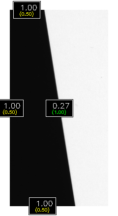

The profile of the intensity of light reflected by the edge, rotated so that it is perfectly vertical, is shown below.  Refer to the earlier link if you are interested in understanding how the ESF can be generated to that level of precision (key word = super-sampling).

The dark portion of the edge is on the left, the bright portion is on the right.  The vertical axis represents raw levels normalized to 16 bit precision, which are proportional to the recorded intensity.  The units of the horizontal axis are the distance center-to-center between contiguous pixels, otherwise known as pixel pitch.  In typical digital imaging sensors the pixels are layed out in a rectangular grid, so pixel pitch is the same horizontally and vertically.  When dealing with units, pixel pitch is often shortened to ‘pixel’, as shown below.

The ESF of a non-existent perfect imaging system should be recorded as a step function in the raw data, with an instantaneous transition from minimum to maximum occurring at the origin. However, blurring introduced by the physical hardware (lens pupil size and aberrations, filter stack, effective pixel aperture and how ‘sharp’ the physical edge is itself) spreads the step out to a monotonically increasing stretched S shape as shown above.   The shorter the rise in pixels, the closer the performance of the lens/camera combination to a perfect imaging system, the better the resulting image ‘sharpness’.   As a first approximation we could arbitrarily say that this lens/sensor/target combination produces the image of an edge on the sensor which rises from 10% to 90% intensity within the space of a couple of pixels (center-to-center = pixel pitch).

ESF to LSF

By taking the differential of the ESF we obtain a Line Spread Function (LSF), equivalent to the one dimensional intensity profile in the direction perpendicular to the edge that a distant, perfectly thin white line against a black background would project on the imaging plane, as captured in the raw data.   If obtained carefully and accurately, the LSF is effectively the projection in one dimension of the two dimensional Point Spread Function (PSF).  This is what makes the math work (more on the theory behind it here).

The  units of the horizontal axis are still the distance between two contiguous pixels in the direction under consideration:

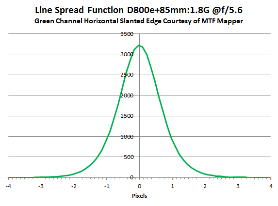
A perfect imaging system and target would record the profile of the line as a spike of vertical intensity at zero pixels only.  In practice that’s physically impossible but clearly the narrower the LSF is spread out in terms of pixels the better its performance.  In this case we could arbitrarily say for instance that one ‘line’  fits within about five pixels, from dark to bright to dark again.  Or we could measure the LSF’s full width at half maximum (FWHM) at 1.7 pixels.

A Line Pair

What would happen on the imaging plane if we had more than one such line, parallel and side by side?  Assuming the lines were the result of incoherent light (mostly true in nature) linearity and superposition would apply so  the aggregate pattern of intensity on the imaging plane would simply be the sum of the individual LSFs, point by point, as represented by the continuous red curve below.  That’s the intensity profile that would be recorded in the raw data from projections of two distant perfectly thin lines against a black background.

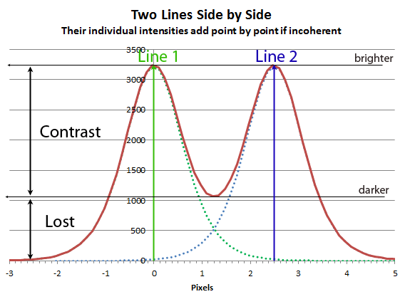
Two lines is one line pair or – interchangeably if you are a person of science – a cycle.  The cycle refers to the bright to dark to bright transitions, in the case of the line pair above it goes peak-to-peak in 2.5 pixels.  Spatially we would say that the period of one cycle (or one line pair) is 2.5 pixels.  Frequency is one over the period so we could also say that the spatial frequency corresponding to this line spacing is 0.4 cycles/pixel ( or equivalently line pairs per pixel pitch).

Clearly the resulting intensity swing from brightest point to darkest point in between the two lines changes depending on how much their line spread functions overlap.    This relative intensity swing is called Michelson Contrast and it is directly related to our ability to see detail in the image.  If no contrast is lost at a specific line spacing (spatial frequency) it means that our imaging system is able to transfer the full intensity swings present in the scene to the raw data.  If on the other hand all contrast is lost (that is our imaging system is only able to record a uniform intensity where originally there was contrast) it means that no spatial resolution information from the scene was captured at that spatial separation/frequency.

The wider the line spread function  and/or the closer the two lines are spaced, the more the overlap and the more the lost contrast – hence the more the lost ‘sharpness’ and the less the detail we are able to discern in the image.

Measuring Response to All Frequencies at Once

The loss of  contrast at decreasing spatial separation – or inversely at increasing spatial frequency – is what the slanted edge method measures objectively and quantitatively for a given target and imaging system set up in one go.   It is able to achieve this feat because an edge is ideally a step function and as we know a step function is made up of all frequencies at once.

Fortunately there is a mathematical operation that will determine the amount of energy present at each frequency once fed intensity functions like our LSF:  the Fourier Transform.  The original signal from the sensor in the raw data is said to be in the Spatial Domain.  After Fourier transformation the result is said to be in the Frequency Domain and often presented as the Power or, in our case, Energy Spectrum of the original signal.

Therefore by taking the Fourier Transform of the LSF as determined above and computing its normalized absolute magnitude (modulus) we obtain the contrast transfer function of the target plus  imaging system in the direction perpendicular to the edge – this is commonly known as its Modulation Transfer Function (MTF).  We take the modulus because MTF is only concerned with the absolute energy present at each spatial frequency, ignoring any phase shifts associated with it.

Interpreting the Modulation Transfer Function

The MTF is normalized to one at the origin by definition.  One means all possible contrast information present in the scene was transferred, zero means no spatial resolution information (detail) was transferred to the raw file.  The MTF curve below shows how much the contrast of a figurative set of increasingly closer ‘lines’ above is attenuated as a function of the spatial frequency (one divided by the given spatial separation) indicated on the horizontal axis.  As we have seen the units of spatial frequency on the sensor are naturally cycles per pixel pitch, or just cycles/pixel for short.

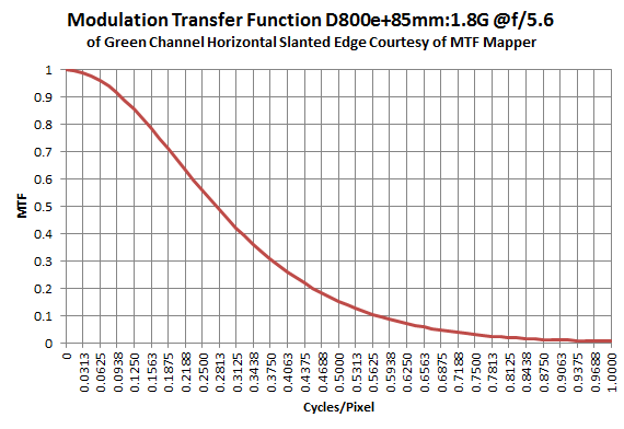
In normal, well setup photographic applications with in-‘focus’ quality lenses, MTF curves of unprocessed raw image data captured with good technique decrease monotonically from a peak at zero frequency (also known as DC).  Zero frequency would occur if the distance between two lines (the period) were infinite –  In such a case no matter how wide each individual line spread function is, the system is assumed to be able to transfer all possible contrast in the scene to the raw data, represented by the normalized value of 1.  For more on the properties of the MTF see the following article on Fourier Optics.

Recall that the MTF curve above is a one dimensional result which only applies in the position on the sensing plane corresponding to the center of the edge, in the direction normal to the edge.

MTF50

One may be interested to know at what spatial frequency the imaging system is only able to transfer half of the possible captured contrast to the raw data.  We can simply read off the curve the frequency that corresponds to an MTF value of 1/2, customarily referred to as MTF50(%).  In this case we can see above that MTF50 occurs when the imaging system is presented with figurative lines of detail alternating at a spatial frequency of about 0.27 c/p (that is the peaks of a line pair are separated by one over that, or about 3.7 pixels).  If one does not have access to the whole curve, MTF50 is considered to be a decent indicator of perceived sharpness when pixel peeping.

The slanted edge method relies on information from the raw data only.  It doesn’t know how tall the sensor is or how far apart the pixels are physically. Without additional information it can only produce the MTF curve as a function of the units for distance it knows: samples at pixel spacing in the raw data. So cycles per pixel pitch (often shortened to cycles/pixel, cy/px or c/p) are the natural units of the MTF curve produced by the slanted edge method.

Converting to Useful Units: lp/mm, lw/ph,…

If we have additional physical information, for instance how far pixels are apart or how many usable pixels there are in the sensor – and we typically do – we can easily convert cycles per pixel pitch into some other useful spatial resolution unit often seen in photography.  For instance the D800e sensor’s pixel pitch is around 4.8um, so 0.27cycles/pixel from the above MTF50 reading  would correspond to 56.3 cycles/mm on the sensor as captured by the given  imaging system:

56.3 cy/mm = 0.27cy/px  / (4.8um/px) * 1000um/mm.

Watch how the units cancel out to yield cycles per mm.  One cycle is equivalent to one peak-to-peak contrast swing – or a line pair (lp).  Units of line pairs per mm (lp/mm) are useful when interested in  how well an imaging system performs around a specific spot of the capture (say the center), in the direction normal to the edge.

But in practice, do 110lp/mm in the center of the small sensor of an RX100III capture represent better spatial resolution IQ (aka ‘sharpness’) in final images viewed at the same size than 56.3lp/mm in the center of a Full Frame D800e capture?

Of course not.   The D800e’s bigger sensor (24mm on the short side) will be able to fit more line pairs along its height than the smaller RX100III’s (8.8mm on the short side).  More line pairs in a displayed image viewed at the same size in the same conditions mean better observed spatial resolution.  Watch again how the units cancel out to yield line pairs per picture height (lp/ph):

D800e = 1351 lp/ph (= 56.3lp/mm * 24mm/ph)
vs
RX100III = 968 lp/ph (= 110lp/mm * 8.8mm/ph).

Units of line pairs per picture height are useful when comparing the performance of two imaging systems apples-to-apples with the final image viewed at the same size.  Picture Height (ph) is used interchangeably with Image Height (ih).

Sometimes line widths (lw) are used instead of line pairs (lp) or cycles (cy).  It’s easy to convert between the three because there are two line widths* in one line pair ( or equivalently one cycle), so 1351 lp/ph correspond to 2702  lw/ph.

The same result could have been obtained simply by multiplying the original measurement in cycles per pixel pitch by the number of pixels on the side of the sensor.  For instance the D800e has 4924 usable pixels on the short side, so in lp/ph that would be

1330 lp/ph = 0.27 c/p * 4924 p/ph [ * 1 lp/c]

which of course would be equivalent to 2659 lw/ph.  The figures are not identical because of slight inaccuracies in the information. The earlier figures rely on the D800e’s pixel pitch being exactly 4.80um and its usable sensor height being exactly 24.0mm, either of which dimension could be slightly off.  The latter figures for picture height are the more precise of the two because they rely only on the number of effective image pixels available for display, which is an accurately known number.

Convention: Landscape Orientation

By convention the displayed image is assumed to be viewed in landscape orientation, so spatial resolution per picture ‘height’ is normally calculated by multiplying by the shorter sensor dimension.  One could make a case that the length of the diagonal should be used instead to somehow level the playing field when aspect ratios differ significantly between sensors – but aspect ratio typically only makes a small difference to the final result so in practice it is often ignored.

Lens aberrations of even excellent lenses vary substantially with direction and throughout the field of view – so MTF should be measured in more than one direction and in various key spots in the field of view in order to determine more completely the actual performance of the imaging system.

In addition some current sensors have anti-aliasing filters active in one direction only, so that MTF can be quite different in one direction versus its perpendicular.  In such cases if the captured detail is not aligned with either direction the spatial resolution performance of the system will vary sinusoidally from maximum to minimum depending on the relative angle of the detail to the strength of the AA.  With a one-directional AA the manufacturer is counting on the fact that detail in natural scenes is typically not all aligned in the same direction so the effective resolution tends to average itself out – though this is often not the case with man-made subjects.

In the face of these many variables the data found on many sites is often the average of perpendicular (tangential and sagittal) MTF readings tested in several spots throughout the field of view.  Read the fine print of each site to figure out where they test and how they aggregate the data.

 

* The use of ‘Line Widths’ is inherited from the post war period (see Duffieux, Kingslake, etc.) when ‘definition’ and ‘resolving power’ were determined by capturing images of something similar to the 1951 USAF target below (wikipedia commons license):

‘Line’ here refers to the  identical bars separated by spaces equal to their width.  So when Kingslake and his cohorts talk about lines per mm they are referring to the number of bars and related spaces within a millimeter.  Since the width of the bars and the width of the spaces that separate them are the same, one cycle is equal to two line widths.  It makes a difference whether the lines are more square or sinusoidal, but to a first approximation the line widths of old and the line pairs described in this article can be assimilated (see for instance Lenses in Photography: The Practical Guide to Optics for Photographers, Rudolf Kingslake, Case-Hoyt Corporation, 1951).