We’ve seen how to model sensors and how to collect signal and noise statistics from the raw data of our digital cameras.  In this post I am going to pull both things together allowing us to estimate sensor IQ metrics: input-referred read noise, clipping/saturation/Full Well Count, Dynamic Range, Pixel Response Non-Uniformities and gain/sensitivity.

There are several ways to extract these metrics from signal and noise data obtained from a camera’s raw file.  I will show two related ones: via SNR in this post and via total noise N in the next.  The procedure is similar and the results are identical.

Sensor Metrics from Measured SNR Curve

Starting with SNR, recall that the performance of a typical Digital Camera can be approximated by the following simplified model, capitals referring to data in DN and lower case letters to quantities in photoelectrons:

(1)  

with S and N  the mean and standard deviation respectively of the uniform measured raw data in units of DN – and s, r and p the signal, read noise and PRNU factor referred to the input of the electronics, all in units of e-.

The highest signal that can be recorded at a given gain (controlled by the in-camera ISO setting) is usually referred to as Full Scale, clipping or saturation.  When using photoelectrons as a unit it is also sometimes improperly called Full Well Count (FWC).  I will use these terms interchangeably.

FWC can be worked into the SNR equation by recognizing that the signal in photoelectrons can be expressed as a factor (x) of the maximum signal

   

with f = FWC in e- if the maximum signal is at clipping.  In this latter case we would say that x = 0.18 when mean signal intensity is 18% of full scale, for instance.  Substituting for s in equation (1) we obtain

(2)  

Formula (2) is of the form y =f(x) because , and are constants for a given sensor setup.  If we assume that a sensor has read noise () equal to 5e-, PRNU () 0.005 and FWC () 50000e- we can construct an SNR curve for such a sensor in a spreadsheet based on our simple model, with normalized signal () from zero to full scale (x = 0 to 1) by using formula (2), as shown below in the solid blue line:

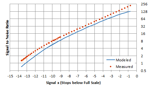
The red dots are actual D810 SNR measurements performed by Jim Kasson and calculated as a ratio of the mean (S) and standard deviation (N) statistics obtained in DN from the green channel raw data at ISO 64 as outlined earlier.  To obtain x in this case we normalize the mean signal  (S) in DN by dividing it by its full scale value, which for  the D810 is 15783 DN at base ISO.

Assuming that the measured data will fit the simple model, all we have to do is vary the values of read noise (r), FWC (f) and PRNU (p) until the modeled curve matches the measured data.  If/when it does we will have estimates for the sensor’s  figures of merit.  We can use  Excel to do the fitting and find the values for us by creating

1. a column with the normalized measured Signal x (shown in log2 format in column T in the figure below);
2. a column with measured SNR from the raw data (column V below); and
3. a column (U) with the modeled values of SNR at every Signal x, based on equation (2) and the three constants  r, f and p (column AA).

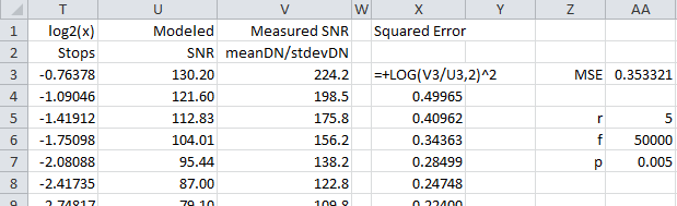
Next introduce a column (X in the figure) that measures the Modeled vs Measured SNR Squared Error at every x, which in this case should be calculated as log2(MeasuredSNR/ModeledSNR)^2, and a cell to collect the mean of the Squared Error column (MSE, in column AA).  Then open Solver, in Excel’s Data tab, and ask it to minimize the MSE cell by varying r, f and p with the fast GRG algorithm.  This is the result:

A very good fit, showing read noise for the green channel of the D810 at base ISO of 4.28e-, FWC of 80322e- and PRNU of 0.  Engineering Dynamic Range can be approximated as the ratio of FWC to read noise, equal to 14.2 stops.  The curve fitting returned a PRNU of zero because the standard deviation data was obtained by subtracting image pairs as described earlier, which minimizes light gradients as well as most non-uniformities and quantization error in this signal range.

If single image standard deviation measurements had been used to create the spreadsheet instead, the model would have returned a very low value for PRNU of around 0.27% and perhaps we would have seen a slight increase in the read noise estimate to the tune of about 1/sqrt(12) summed in quadrature: the uniform quantization error, minimized earlier by pair subtraction.

All we are left to determine is the gain at this ISO, which can be easily calculated by taking the ratio of full scale in DN to FWC in e- = 15783 / 80322.  So gain g = 0.1965 DN/e- and sensitivity k = 5.09 e-/DN.  Our sensor’s noise performance in the green channel has been characterized at base ISO.  The SNR PTC is my favorite way to estimate these parameters because it shows that all one needs to estimate input-referred figures of merit in e- for a digital sensor like read noise, FWC, Dynamic Range and more is a good set of mean and standard deviation measurements in DN from the raw data.

Next, how to do the same thing by plotting a different Photon Transfer Curve, mean signal versus its standard deviation in DN.