Connecting Photographic Raw Data to Tristimulus Color Science

Absolute Raw Data

In the previous article we determined that the three $r_{_L}g_{_L}b_{_L}$ values recorded in the raw data in the center of the image plane in units of Data Numbers per pixel – by a digital camera and lens as a function of absolute spectral radiance $L(\lambda)$ at the lens – can be estimated as follows:

(1) $\begin{equation*} r_{_L}g_{_L}b_{_L} =\frac{\pi p^2 t}{4N^2} \int\limits_{380}^{780}L(\lambda) \odot SSF_{rgb}(\lambda) d\lambda \end{equation*}$

with subscript $_L$ indicating absolute-referred units and $SSF_{rgb}$ the three system Spectral Sensitivity Functions. In this series of articles $\odot$ is wavelength by wavelength multiplication (what happens to the spectrum of light as it progresses through the imaging system) and the integral just means the area under each of the three resulting curves (integration is what the pixels do during exposure). Together they represent an inner or dot product. All variables in front of the integral were previously described and can be considered constant for a given photographic setup.

The Connection to Luminance and Exposure

Radiance $L_e$ represents the sum (or the integral) of the power contributed by every small constant-width wavelength interval of spectral radiance $L(\lambda)$ within the visible spectrum. It has units of $W/sr/m^2$ .

In Color Science and photography the corresponding photometric quantity is Luminance $L_v$ with watts $W$ in the units of radiance replaced by lumens $lm$ . lumens are just watts as perceived by the Human Visual System, which has spectral efficiency $V(\lambda)$ , see Figure 1 below. Since in the SI System $lm/sr$ is a candela ( $cd$ ), the total luminance $L_v$ contained in the visible wavelength range is usually expressed in $cd/m^2$ – a unit photographers are familiar with:

(2) $\begin{equation*} L_v = K_m \int\limits_{380}^{780} L(\lambda)\odot V(\lambda) d\lambda, \text{ $cd/m^2$} \end{equation*}$

where $V(\lambda)$ is the Standard Observer photopic luminous efficiency function shown in Figure 1 below and $K_m$ is the luminous efficiency conversion constant, about 683.002 lm/W.^[1]

For instance, if radiance $L(\lambda)$ were equal to a spectrally flat stimulus of 1 $mW/sr/m^2/nm$ , Luminance $L_v$ would be equal to 77.2 $cd/m^2.$

It is obvious that if one of the Spectral Sensitivity Functions in Equation (1) were equal to $V(\lambda)$ then by definition the respective integral would resolve to Luminance $L_v$ . Taking the area of a pixel $p^2$ out of the equation, we would have for the given channel

(3) $\begin{equation*} H_v = \frac{\pi}{4} \frac{t}{N^2}L_v, \text{ $lx$-$s$} \end{equation*}$

which if $L_v$ is in $cd/m^2$ is the equation for photographic Luminous Exposure $H_v$ in $lx$ – $s$ – for a camera and lens in the center of the field of view, ignoring in this context vignetting and lens transmission losses since we said that $L(\lambda)$ here represents radiance at the front of the lens . This is the basis of the Exposure Value system.

For instance with shutter speed $t$ = 1/30 of a second, f-number N = 4 and $L_v$ as above, Exposure $H_v$ would be equal to 0.1263 $lx$ – $s$ . For reference, many digital cameras today start to clip around one $lx$ – $s$ at ISO 100 in the raw data.

The Connection to Tristimulus XYZ Color Space

Conveniently it turns out that the $\bar{y}(\lambda)$ Color Matching Function of the CIE 2° Standard Observer is in fact chosen to be identical or very similar to $V(\lambda)$ , as can be seen in Figure 1 below. This is the reason why the $Y$ channel in the CIE XYZ color space is often referred to as Luminance. Ideally it is Luminance, mostly relative but possibly absolute.

This tidbit reminds us that one of the central tenets of photographic Color Science is projecting spectral distributions $L(\lambda)$ to the tristimulus $XYZ$ color space as follows:

(4) $\begin{equation*} XYZ = K \int\limits_{380}^{780}L(\lambda) \odot CMF_{xyz}(\lambda) d\lambda \end{equation*}$

with $K$ an appropriately chosen constant and $CMF_{xyz}(\lambda)$ the three CIE Color Matching Functions $\bar{x}(\lambda)$ , $\bar{y}(\lambda)$ and $\bar{z}(\lambda)$ in turn. The integral, typically replaced by discrete summation in practice, results in one value for each of the three curves, designated in turn as tristimulus value $X$ , $Y$ and $Z$ .

color matching luminous efficiency functions — Figure 1. CIE (2012) 2° XYZ “physiologically-relevant” Color Matching Functions and photopic Luminous Efficiency Function (V) from cvrl.org, the Colour & Vision Research Laboratory at UCL. The items in the legend refer to CMF_X, CMF_Y and CMF_Z in the text respectively. After normalization to unit area the set of curves is scaled for display so that Y = V peaks at 1.

Clearly if $K$ is made equal to the luminous efficiency conversion constant, 683.002 lumens/watt, then $Y$ is Luminance in $cd/m^2$ by definition, per Equation (2).

On the other hand in imaging it is typically more convenient to choose $K$ so that $Y$ becomes equal to 1 (or 100%) when $L$ represents the spectrum of brightest diffuse white under the given illuminant. We accomplish this by making $K$ the inverse of Luminance from a perfect diffuser $L_{mdw}(\lambda)$ , reflecting or transmitting the spectral distribution of the illuminant

(5) $\begin{equation*} K_{Y} = \frac{1}{\int L_{mdw}(\lambda)\odot \bar{y} \text{ }d\lambda} \end{equation*}$

Here $K_Y$ is a single scaler and $_{mdw}$ stands for maximum diffuse white.

CIE CMFs are Area Normalized to Begin with

$CMF_{xyz}$ in this article represents the CIE (2012) 2-deg XYZ “physiologically-relevant” color matching functions, fine tuned over decades of psychophysical testing with live Observers – we will drop the $_{xyz}$ and $_{rgb}$ subscripts in $CMF$ and $SSF$ from now on not to clutter the relative equations, just remember that they represent three curves each.

When used with Equation (4) they are the most important functions in colorimetry because if two spectral stimuli result in the same $XYZ$ tristimulus values they should look the same to the average Observer. And if they are sufficiently different they should look different.

Note that the $CMF$ curves in Figure 1 are in arbitrary units, meaning that they have been normalized individually so that their areas are all equal under flat spectral radiance, aka equi-energy stimulus $Se$ . They have also been all scaled by a common factor so that $\bar{y}(\lambda)$ peaks at one, just like luminous efficiency function $V(\lambda)$ does. It is clear however that this scaling becomes irrelevant after the normalization provided by $K_{Y}$ in Equation (5): for instance under maximum diffuse equi-energy stimulus the tristimulus values for $XYZ$ will be [1 1 1], Standard Illuminant $S_e$ ‘s so-called White Point as we are used to seeing it in imaging.

SSFs are Area Normalized by White Balancing

To make the two sets of functions intuitively comparable, Spectral Sensitivity Functions can also be normalized so that the areas under their curves are all equal to one for radiance from the illuminant after maximum diffuse reflection, $L_{mdw}(\lambda)$ . Unlike for $CMF$ , however, the areas under the three $SSF$ curves of our imaging systems are not usually presented equal to start with, so this time we achieve the objective by dividing each function by the area under its own curve

(6) $\begin{equation*} K_{rgb} = \frac{1}{\frac{\pi p^2 t}{4N^2} \int L_{mdw}(\lambda) \odot SSF(\lambda) d\lambda} \end{equation*}$

Collecting that normalization and all constants in Equation (1) into $K_{rgb}$ we see that it evaluates to three scalars under the given spectral radiance, one each for the $\bar{r}(\lambda)$ , $\bar{g}(\lambda)$ and $\bar{b}(\lambda)$ functions of the $SSF$ . These are the multipliers that are applied to the respective $rgb$ color channel as part of the operation normally referred to as ‘white balance‘ during raw conversion.

The normalized forms of Equations (1) and (4) allow us to concentrate on the shape and position of the individual functions as opposed to their amplitude. This is what the Spectral Sensitivity Functions of the Nikon D5100 camera and lens shown at the bottom of the last article look like after normalization by $K_{rgb}$ under equi-energy stimulus $S_e$ (scaled, for comparison only, by the same CIE factor as CMFs were subjected to in Figure 1):

Figure 2. Area normalized Spectral Sensitivity Functions of a Nikon D5100 with an unknown lens as measured by Darrodi et al at the National Physical Laboratory, London, here scaled so that CMF_Y in Figure 1 and SSF_G have the same area. Legend items refer to SSF_R, SSF_G and SSF_B in the text respectively.

Trichromatic Equation (1), producing $rgb$ raw values, then takes the same form as Equation (4), producing $XYZ$ tristimulus values:

(7) $\begin{equation*} rgb = K_{rgb}\int\limits_{380}^{780} L(\lambda)\odot SSF(\lambda) d\lambda \end{equation*}$

The $rgb$ raw values produced by Equation (7) under maximum diffuse $S_e$ will then also be equal to [111] after normalization by $K_{rgb}$ , as seen in Figure 3 below.

In fact they will always be [1 1 1] after white balance independently of the illuminant in $L_{mdw}$ because we defined $K_{rgb}$ as a function of all three $\bar{r}$ , $\bar{g}$ , $\bar{b}$ curves. This is not the case for $XYZ$ values normalized by single scalar $K_Y$ – so while $Y$ will be equal to one after normalization, $X$ and $Z$ will vary with the illuminant. Their values will be those of the illuminant’s White Point.

We are now firmly in the relative domain, having scaled each CMF and SSF curve individually at will, effectively giving up on absolute values. This is ok because the curves are linearly independent (they are not mixed – yet) and because working with relative units simplifies the process considerably in photography.

Maximum Diffuse White at $Y$ = $g$ = 1

So for a given spectral radiance from the scene we get two sets of triplets: CIE $XYZ$ tristimulus reference values per equation (4), and $rgb$ trichromatic raw data per equation (7). The absolute energy of radiance $L(\lambda)$ determines the linear range of responses in both systems, which under standard normalizations go from a minimum value of 0 with no light to a value of 1 in the $Y$ and $g$ channels with maximum diffuse white $L_{mdw}(\lambda)$ as the stimulus.

One is sometimes taken to mean 100(%) in Color Science, in which case the range of values to diffuse white is shown from 0 to 100 instead of from 0 to 1. In image processing it is more convenient to use 1 because it simplifies the math, so that’s what we’ll do here.

Photographers and automatic exposure meters typically attempt to choose parameters for their captures that will result in maximum diffuse white landing somewhere around full scale in the raw data – so $rgb$ intensities at clipping, say around 15000 $DN$ for a current bias-subtracted 14-bit camera, get normalized to 1 by $K_{rgb}$ . Continuing the previous example, assuming a typical digital camera that clips around 1 $lx$ – $s$ at ISO100, we would then expect raw data around 12.6% of full scale with Luminance of 77.2 $cd/m^2$ from the earlier example.

Unattainable Perfect Color

For ‘exact’ CIE color the response of the imaging system, $rgb$ raw intensities, should mimic as closely as possible $XYZ$ values under the same stimulus. It is useful to normalize $CMF$ and $SSF$ by $K_{Y}$ and $K_{rgb}$ , shown as $CMF'$ and $SSF'$ below respectively, because it brings them to a similar scale and makes them easier to compare visually. Equations (4) and (7) would then ideally produce identical results:

(8) $\begin{equation*} \int\limits_{380}^{780} {L(\lambda)\odot CMF'(\lambda) d\lambda= \int\limits_{380}^{780} L(\lambda)\odot SSF'(\lambda) d\lambda \end{equation*}$

with $'$ indicating normalization as discussed. Clearly if $SSF'(\lambda)$ were identical to $CMF'(\lambda)$ we would have perfect color out-of-camera. But it is obvious by comparing their plots under equi-energy stimulus $S_e$ below that the two sets of normalized curves have quite different shapes and also appear somewhat shifted with respect to one another.

Figure 3. Left: CIE (2012) XYZ “physiologically relevant” Colour Matching Functions sampled every nm; they are scaled by the same factor so that the ybar curve results in Y = 1 under illuminant S_e. Right: Nikon D5100 with unknown lens Spectral Sensitivity Functions, sampled every nm, each curve normalized so that the area under each curve also adds to 1 under the same stimulus.

On the other hand there are, not coincidentally, some similarities: both sides of Equation (8) resolve to [1 1 1] under equi-energy illuminant $S_e$ ; the curves are all mostly contained in the 400-700nm wavelength range; and each curve has a main peak more or less spaced out from the others (the second minor hump in $\bar{x}(\lambda)$ is a byproduct of the math, see the next article).

I have never seen $SSF'$ that look exactly like $CMF'$ in current consumer cameras, in part because of physical limitations of sensors like saturation and noise; and the fact that they need to be able to work in many different conditions, such as in candle light (much more red energy than blue) as well as on a bright sunny day on a Nordic glacier (vice versa).

In order to minimize the possibility of clipping and/or noise in $rgb$ , it is usually useful to have a more efficient green channel in the center acting like the fulcrum of a seesaw – with weaker red and blue at either end moving up and down in opposite directions depending on scene and illuminant (refer to Figure 4 in the previous article). This forces other compromises that result in $SSF$ curves different in shape and more spread out than the ideal.

Let’s Compromise

So next best is to try to minimize differences between the two sets of three curves: since the system is assumed to be linear, it should be possible to obtain an improved approximation to $CMF'$ by using a linear combination of the three $SSF'$ under a given spectral stimulus. Linear algebra tells us that we can find a 3×3 matrix $M$ that minimizes the square of differences between the resulting curves so that approximately

(9) $\begin{equation*} L(\lambda)\odot CMF' \approx M * [L(\lambda)\odot SSF'(\lambda)] \end{equation*}$

with $*$ indicating matrix multiplication. Absolute radiance can be replaced by relative spectral radiance $L'(\lambda)$ because $L(\lambda)$ appears on both sides of Equation (9) so its absolute strength cancels out: what remains is just its spectral signature, often normalized for convenience. For instance if it represents just irradiance from the the light source it is often normalized to have a value of one at the mean wavelength in the working range, or alternatively 560nm.

After pixel integration we get the equivalent of Equation (8)

(10) $\begin{equation*} \int\limits_{380}^{780} {L'(\lambda)\odot CMF'(\lambda) \approx M * \int\limits_{380}^{780} L'(\lambda)\odot SSF'(\lambda) \end{equation*}$

$d\lambda$ ‘s omitted because they can be assumed to be the same (and to make the Equation fit on one line:). Equation (10), based on triplets of trichromatic values, is looser and more forgiving than Equation (9), which instead works on full spectra – because it also allows for metamers. For a given camera and set of Spectral Sensitivity Functions we can solve for $M$ as a function of the relative spectral radiance $L'(\lambda)$ at the lens:

(11) $\begin{equation*} M_{(L'_{\lambda})} = [L'(\lambda) CMF'(\lambda)] * [L'(\lambda) SSF'(\lambda)]^{-1} \end{equation*}$

with $^{-1}$ the inverse of the array in the square brackets and $*$ matrix multiplication. The other products are either element-wise or ‘dot’ depending on whether Equation (9) or (10) is applied respectively. Clearly the resulting matrices will be similar but not exactly equal in either case, having minimized two slightly different functions from the same set of data: least square wavelength-by-wavelength differences between the curves themselves vs differences between the relative integrated tristimulus values.

Note that there would also be a closed form solution for matrix $M$ even if we hadn’t normalized $CMF$ and $SSF$ curves by their respective constants $K_{Y}$ and $K_{rgb}$ – the matrix would simply absorb the constants and work happily with the functions as they are before normalization (as we will see in the article on Linear Color Transforms).

Transform matrix $M$ above is optimized for the spectral distribution of one radiance only, $L'(\lambda)$ . Assuming flat spectral stimulus $S_e$ at the lens and applying Equation (11) with full spectra, matrix $M_{(S_{e})}$ for the D5100 with unknown lens in Figure 2 would be

Using that matrix to project the relative $SSF'$ to the $XYZ$ connection color space, this is how close (or not) its curves come to the respective $CMF'$ :

Nikon D5100 Spectral Sensitivity Functions in XYZ — Figure 4. CIE 2deg CMFs (solid curves) and given SSFs (dotted) projected to XYZ by matrix multiplication, assuming just spectrally flat stimulus Se and the same scaling as Figures 1 and 2 for comparison only.

The projected green curve $\bar{g}$ does a decent job of staying close to its $\bar{y}$ counterpart, the other two less so. Of course some system SSFs are better than others. In 2012 Jun Jiang et al at the Rochester Institute of Technology measured the Root Mean Square Error resulting from 28 digital camera SSFs with unknown lenses, early Canons did better than most.^[2]

Locally Generalized Compromises

More in general, and more relevant to photography, we can obtain matrices optimized for specific scene types and light source combinations – say sunny spring mountain landscapes – by generating a set of radiances $L'_n(\lambda)$ based on a number of expected principal reflectances $R_n(\lambda)$ at the scene under one illuminant at the time. Recall that luminance $L$ is reflected illuminance $E$ so that

(12) $\begin{equation*} L'_n(\lambda) = E'(\lambda) \odot R_n(\lambda) k_n \end{equation*}$

where $E'(\lambda)$ is the relative Spectral Power Distribution of the illuminant at the scene (normalized to one at 560nm), $R_n(\lambda)$ the $n$ principal diffuse reflectances expected in such a scene (in % spectral efficiency) and $k_n$ constants that we can drop because we are only interested in normalized $L'_n(\lambda)$ which appears on both sides of the relevant equations.

By applying Equation (11) repeatedly to each $L'_n(\lambda)$ expected at a scene type we can generate a mean single compromise color matrix, call it $M_{(L'_{n\lambda})}$ , that minimizes potential errors for that scene under the chosen illuminant. Such compromise matrices can be calculated for specific applications like landscapes, studio or non studio portraits, art reproduction, B&W etc. Tellingly, similarly named camera profiles are often found in current raw converters.

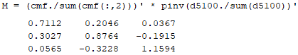
Using the 24 reflectances of an X-Rite ColorChecker target as measured by BabelColor^[3] , matrix $M_{(L'_{n\lambda})}$ from full spectra for the previously mentioned Nikon D5100 and unknown lens under standard illuminant $S_e$ would be

Such Compromise Color Matrices can be easily generated for other illuminants and sets of reflectances, as can be deduced from the short Matlab/Octave example linked in the notes below.^[4]

With $M_{(L'_{n\lambda})}$ in hand for the expected radiance mix, $XYZ$ tristimulus values can be approximated as follows from captured $rgb$ demosaiced raw data normalized as discussed earlier,

(13) $\begin{equation*} XYZ \approx M_{(L'_{n\lambda})} * rgb \end{equation*}$

where data triplets are in 3xN column vector notation and $*$ indicates matrix multiplication. Equation (13) works just as well on trichromatic vs the respective full spectral data of Equation (10) because of the distributive property of multiplication.^[5] If we keep track of all the constants we can obtain approximate results in absolute units $X_LY_LZ_L$ , although this is not necessary in photographic imaging.

An Aside

Matrices obtained by minimizing the square difference between spectral or trichromatic data can be used to convert $rgb$ raw data triplets to $XYZ$ tristimulus values because what is good for the 31+ Dimensional goose is good for the 3D gander.^[6] However, minimizing errors between the two sets of curves without taking into consideration the different color sensitivity of the Human Visual System throughout the spectrum may not be the best way to obtain optimal perceptual results.

For instance the attentive reader may have noticed by summing up the respective rows that neither matrix presented above results in the expected white point for a neutral input of [1 1 1], both having the objective of minimizing the sum of square errors in the mix of spectral radiances instead. Though this approach may result in smaller overall deviations between the curves, it can produce the appearance of objectionable color casts. More controlled and relevant results can be had by constrained regression^[7] and by using well established perceptual color difference metrics, as outlined in the Color Transform article.

She may also have wondered why try to mimic the bumpy, synthetic $XYZ$ color space instead of one with more affinity to the physical world, such as the Long, Medium and Short $LMS$ space where Cone Fundamentals reside. Next.

Notes and References

_{1. A description of the photopic Luminosity Function can be found here.

2. Jun Jiang, Dengyu Liu, Jinwei Gu and Sabine Susstrunk. What is the Space of Spectral Sensitivity Functions for Digital Color Cameras?. IEEE Workshop on the Applications of Computer Vision (WACV), 2013.

3. The BabelColor page with the Excel spreadsheet containing the 24 spectral reflectances of pre-2014 ColorChecker24 targets, measured and averaged over 30 samples with different instruments, can be found here.}_{4. The routine used to estimate a Compromise Color Matrix given SSFs, CMFs and expected illuminant and reflectances at the scene can be downloaded by clicking here.

5. It is easy to prove to oneself that the distributive property of multiplication implies that multiplying spectral curves by matrix M and then summing the result into a triplet is the same as summing the curves first and then multiplying the resulting triplets by M.

6. Just like the tristimulus and raw value triplets can be considered to constitute unique vectors representing color in 3D XYZ and RGB coordinate systems, continuous spectra can be considered to be vectors of infinite length/dimensions. In practice it usually suffices to sample the visible wavelengths at least every 10 nm. So sampling a given spectral curve at a minimum from 400 to 700nm every 10nm results in a vector of at least 31 values/dimensions.

7. For constrained regression resulting in white point preserving matrices see for instance Finlayson, Graham D. and Mark S. Drew: “White-Point Preservation Enforces Positivity.” Color Imaging Conference (1998).

8. In this article guidance and solace came from Hunt’s excellent book: Measuring Color, Third Edition, R.W.G. Hunt. Fountain Press, 1998.}

Strolls with my Dog

Connecting Photographic Raw Data to Tristimulus Color Science

Absolute Raw Data

The Connection to Luminance and Exposure

The Connection to Tristimulus XYZ Color Space

CIE CMFs are Area Normalized to Begin with

SSFs are Area Normalized by White Balancing

Maximum Diffuse White at $Y$ = $g$ = 1

Unattainable Perfect Color

Let’s Compromise

Locally Generalized Compromises

An Aside

Notes and References

Leave a Reply Cancel reply

Musings about Photography

Absolute Raw Data

The Connection to Luminance and Exposure

The Connection to Tristimulus XYZ Color Space

CIE CMFs are Area Normalized to Begin with

SSFs are Area Normalized by White Balancing

Maximum Diffuse White at = = 1

Unattainable Perfect Color

Let’s Compromise

Locally Generalized Compromises

An Aside

Notes and References

Want to share?

Leave a Reply Cancel reply

Musings about Photography

Maximum Diffuse White at $Y$ = $g$ = 1