Photons, Shot Noise and Poisson Processes

Every digital photographer soon discovers that there are three main sources of visible random noise that affect pictures taken in normal conditions: Shot, pixel response non-uniformities (PRNU) and Read noise.^[1]

Shot noise (sometimes referred to as Photon Shot Noise or Photon Noise) we learn is ‘inherent in light’; PRNU is per pixel gain variation proportional to light, mainly affecting the brighter portions of our pictures; Read Noise is instead independent of light, introduced by the electronics and visible in the darker shadows. You can read in this earlier post a little more detail on how they interact.

However, shot noise is omnipresent and arguably the dominant source of visible noise in typical captures. This article’s objective is to dig deeper into the sources of Shot Noise that we see in our photographs: is it really ‘inherent in the incoming light’? What about if the incoming light went through clouds or was reflected by some object at the scene? And what happens to the character of the noise as light goes through the lens and is turned into photoelectrons by a pixel’s photodiode?

Fish, dear reader, fish and more fish.

Emitting Photons

While studying natural light sources like blackbody radiators (a star, the sun or, to a decent approximation, a tungsten light bulb) Planck and Einstein figured over 100 years ago that emitted light energy appeared not to be continuous – but to be quantized, in the form of energy packets now referred to as photons.

Figure 1. Simulation of the quantized, random nature of light emission and travel. After a usually long journey, photons emitted randomly and independently at a constant rate are bounced around, deflected and blocked. Those that eventually funnel into our lenses are hopefully collected by pixels in our digital camera sensor.

Physicists have been arguing about this figuring ever since (see wave/particle duality) but in the context of digital photography particles are a convenient match to observations in the raw data – so particles it is.

If we look at a lightbulb we do not see the individual photons: they are too many and too closely packed together. What we see instead is the average (the mean) intensity of their stream as they hit our eyes. Assuming the bulb’s power supply is steady, so will be its perceived output.

The energy packets of light are emitted at a certain steady rate by the source, for instance at the rate of 30 watts. Watts is short for joules per second, with joules the units of energy. Watts can be expressed as a certain number of photons per second when the spectral power distribution of the light is known (see for instance the article on blackbody emission).

However, even though the source may produce photons at a certain constant rate, they are apparently not emitted at the exact same number per given interval of time and/or space. Quite the contrary, physicists surmised that they can be considered to be emitted in the direction of our lenses independently of each other and completely randomly as a stochastic process. Though to keep up with the given rate, the production of photons needs to chug along appropriately.

Time, Space and (Shot) Noise

In what follows we consider what happens to photons reaching a uniformly illuminated area on an imaging sensor during a certain period of time (referred to as Shutter Speed or Exposure Time in photography). Because of the random nature of photon emission and arrival, it makes no difference whether we consider a single pixel on the sensor over multiple periods of time – or several neighboring pixels during a single interval. Statistically, the two scenarios are exactly equivalent as long as the mean rate of arrival is constant.

So if you were a pixel in a monochrome digital camera sensor exposed to a uniform light source like in Figure 2, you would see photons arriving at the same mean rate as your neighbors. However, since photons were emitted and arrived at random times, some pixels would see more of them than others over a given period. For instance, if Exposure were between 4.5 and 5 arbitrary time units in the figure below, there would be quite a variation from pixel to pixel (count them).

Figure 2. A snapshot in time of photon flow.

In other words, if we captured a uniformly illuminated, perfectly smooth diffuse reflector like a gray card in raw data with a monochrome camera and looked at it with a tool like RawDigger,^[2] we would see intensity fluctuating around a mean from pixel to pixel.

We refer to the mean as the Signal; and these fluctuations from the mean as ‘Noise‘ – because they look like grain in our pictures. In this case we would call it ‘Shot Noise’, partly because the random nature of the arrivals results in a pattern similar to that produced in the center of a shot gun target (see an example here looking very much like Figure 2). In visible-light imaging the term Photon Shot Noise, or just Photon Noise, is often used when photons are involved.^[4]

A measure of fluctuations from the mean is the Standard Deviation. It turns out that the mean to standard deviation ratio of such raw data (the so-called Signal to Noise ratio, SNR) correlates well with our perception of how noisy an image is.

Random Arrivals at a Given Rate …

So what distribution of photon arrivals could we expect from radiance in the direction of our sensor, made up of an independent and random number of photons, though at a constant known rate in space and time? Say that during a given exposure time our 30W light bulb generated 104,000 photons uniformly towards a patch of 200×100 pixels (20,000). What range of photon arrivals could the pixels see during Exposure?

Since arrivals are independent, random, at a constant known rate and all pixels are the same size (a uniform, stationary process) we would expect an average signal of 5.2 photons per pixel (104/20) for our Exposure – but what about the fluctuations? It’s easy enough to try it out numerically from first principles: generate 104k floating point random numbers between 0 and 20,000; and record how many fall into each integer slot, representing a pixel (or equivalently a uniform non overlapping period of time). Here is a Matlab/Octave script that does just that:^[8]

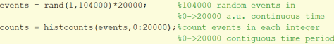
Then add up the number of pixels with the same photon count and plot the resulting histogram, as shown below in blue (ahem):

Figure 3. Blue: Histogram of 20,000 random numbers generated with a mean rate of 5.2 events per slot. Brown: Histogram of Matlab’s poissrnd function for 20,000 numbers with a mean of 5.2. The two histograms practically overlay each other.

What do you know, it looks like a Poisson mass function with mean of 5.2.

… = Poisson Distribution

Statistics 101 tells us that when we count

independent events
random in time and space
arriving at a constant rate

over a given period the result is a Poisson distribution. And in fact Matlab’s built-in Poisson distributed random number generator (poissrnd) reproduces these counts almost exactly,^[3] as can be seen by the brown overlaid histogram above.

The asymmetrical histogram shape makes some intuitive sense, since the rate of arrival at 5.2 per pixel is close to the origin, which precludes symmetry since the number of counted events can only be nonnegative integers by definition (the minimum count is zero). As the mean rate increases, the left tail of the distribution approaches zero probability farther and farther from the origin and the Poisson distribution looks more and more symmetrical, until it can effectively be approximated by a Gaussian with similar mean and standard deviation (the black curve in the Figure below).

Figure 4. Discrete Poisson (blue bars) vs continuous Gaussian (black line) distributions with the same mean. From: https://www.durham.ac.uk/departments/academic/physics/labs/skills/poisson-distribution/

Relevant Properties of a Poisson Distribution

A Poisson distribution describes the probability ( $p$ ) of a certain number of arrivals ( $i$ ) for a specified constant rate of arrivals ( $s$ )

(1) $\begin{equation*} p(i) = e^{-s}\cdot \frac{s^i}{i!} \end{equation*}$

Equation (1) is the well known Poisson Probability Mass Function.

In photography $\bfseries{s}$ can be thought of as a certain number of photons per unit area per unit time (for instance per $\mu m^2$ per second), a quantity known by the name of irradiance or illuminance. If we integrate it (count it) over a given period, say exposure time, $s$ represents a number of photons per unit area, which we refer to as Exposure. We normally think of it as ‘the signal’ as it reaches silicon and then propagates ideally linearly through the electronics, all the way to the raw file.

Continuing with the data related to the empirical example in Figure 3, which has a mean Exposure of 5.2000 photons per pixel, the probability that a specific pixel collect 3 photons is

$p(3) = e^{-5.2}\cdot \frac{5.2^3}{3!} = 12.93\%.$

12.93% of 20,000 pixels is 2586. This is confirmed by the relative bin count, which shows 2560 pixels with a count of 3, within the 1% error band predicted by propagation of errors for 20,000 samples (as discussed at the bottom of this article).

One of the key properties of a Poisson distribution is that for a given mean rate (signal $s$ ) the standard deviation of random arrivals (shot noise $\sigma_s$ ) is equal to the square root of the signal

(2) $\begin{equation*} \sigma_s = \sqrt{s} \end{equation*}$

or 2.2804 in the case of our example with a 5.2000 mean rate. The empirical data used in Figure 3 resulted in a standard deviation of 2.2882, also within 1% of theory.

Consequently, the perceptually relevant photon Signal to Noise Ratio is

(3) $\begin{equation*} SNR = \frac{s}{\sigma_s} = \frac{s}{\sqrt{s}} = \sqrt{s}, \end{equation*}$

which means that in the absence of noise sources other than shot noise, signal $s$ can be estimated by $SNR^2$ . In our case it would be (5.2000/2.2882)^2 = 5.1644, again within 1% of the original signal, as expected given the number of samples. This property is the basis for Photon Transfer Curves and has neat practical implications that we have explored elsewhere.^[4]

Cloud, Lens Transmission and Object Reflectance

So assuming they are in its line of sight, photons are emitted randomly and independently at a certain rate from the source and hence arrive with a Poisson distribution at the detector (an eye, a sensor). What happens to their distribution if they first have to go through a cloud or a lens?

Thinking about the monochromatic case first, and assuming that the role of the, say, cloud is to randomly scatter some photons away from the detector, it makes intuitive sense that the photon distribution be Poisson even after scattering has taken place. In fact, if you eliminate random photons from those arriving randomly, you are left with fewer, independent, randomly arriving photons (random – random = random, right?) – so still satisfying the three conditions of a Poisson distribution, albeit clearly at a lower constant rate.

Any process that randomly divides incoming independent events into two classes – some that are blocked / deflected / reflected / absorbed / etc.; and the rest that continue on – is a Binomial process. And based on the discussion just above we now realize that Poisson arrivals still result in a Poisson distribution after having interacted with a Binomial process, as better explored further down.

Polychromatic Random Arrivals at a Given Rate

If the light is not monochromatic and the removal function shows a varying spectral response, like a lens color cast or the Spectral Sensitivity Functions of the Color Filter Array, then photons of different energies will be affected differently. In other words, pretend breaking the spectral distribution of arriving photons down into many independent contiguous monochromatic slivers of increasing frequency (hence energy). The behavior in each frequency band (or equivalently wavelength) will be as described above for the monochromatic case, therefore it will result in an observable Poisson distribution, each with its own mean signal and standard deviation equal to the square root of the mean.

Since they are statistically independent, adding up the distributions of all monochromatic bands results in the polychromatic Poisson distribution, with aggregate mean equal to the sum of the individual means and standard deviation equal to the square root of the aggregate mean.

This is obviously also true after photons arriving at the sensor have gone through a Bayer CFA: in the absence of other sources of noise, the raw data under each $\bar{r}\bar{g}\bar{b}$ uniformly illuminated color filter will show a Poisson distribution.

So this is why we observe photon noise with a Poisson distribution even after the relative light has been bouncing around and filtered by the physical world for a while. What happens when it hits silicon? More of the same.

Photoelectric Effects

We will use the photoelectric effect as an example of a Poisson distribution interacting with a Binomial process, as described earlier. Einstein first described the photoelectric effect in 1905, where photons striking certain materials are absorbed by them, possibly resulting in the freeing of photoelectrons which, when collected, produce a measurable current (the units of current can be expressed as a certain number of electrons per second). The significance for photographers is that with digital image sensors the current from every pixel during Exposure is eventually converted into Data Numbers and stored into the camera’s raw file.

Figure 5. Photons interacting with silicon free electrons that can be collected, thus generating a current. Image by Ponor under license.

As Janesick clearly explains in his aptly named book on Photon Transfer,^[4] only photons of a certain energy incident on a semiconductor will interact with its atoms. Imaging sensor photodiodes are usually made of silicon, which is transparent to photons with wavelengths greater than about 1000 $nm$ , beyond the near infrared.

On the other hand wavelengths shorter than 1000 $nm$ have a chance of interacting with silicon atoms, dislodging photoelectrons to be collected in the photodiode’s well. The probability of that happening is denoted interacting Quantum Efficiency (or just QE in photography). Thus

(4) $\begin{equation*} QE = \frac{\text{average photoelectrons generated}}{\text{average interacting photons}} \end{equation*}$

In the 380-780nm visible range of interest to photographers, only one photoelectron is effectively freed for each photon interaction that occurs, independently of the energy of the photon. Below about 400nm, the more energetic photons can cause multiple electrons to become free, but we will ignore this possibility here since in practice most cameras used in digital photography have UV/IR cut filters that block photons at those energies.

So in digital photography we don’t have to worry about photons not interacting or generating more than one photoelectron: for all practical purposes in the wavelength range of interest Quantum Efficiency is the mean number of generated photoelectrons ( $e$ ) divided by the mean number of interacting photons ( $s$ )

(5) $\begin{equation*} QE = \frac{e}{s}. \end{equation*}$

Conversely, if we know QE, the number of interacting photons can be estimated by dividing the mean number of resulting photoelectrons by QE.^[5]

Poisson → Binomial = Poisson Distribution

Therefore after bouncing around and being filtered, photons from the scene arrive randomly and independently at the sensor, with a certain constant mean rate $s$ , photon noise equal to standard deviation $\sigma_s$ and a Poisson distribution. Every such photon then has a probability equal to Quantum Efficiency of generating a photoelectron. The mean signal after interacting with silicon is then by definition

(6) $\begin{equation*} e = s \cdot QE \end{equation*}$

with $e$ the mean number of photoelectrons generated.

Multiplying the values of a random sample by a constant causes the original mean and standard deviation to be multiplied by the same constant – so one might think that the standard deviation resulting from Poisson arrivals after QE would just be photoelectrons with mean as above and standard deviation equal to the incoming one times $QE$ :

(7) $\begin{equation*} \sigma = \sigma_s \cdot QE = \sqrt{s} \cdot QE. \end{equation*}$

However, that’s not the case here: when there are a number of events, each with probability QE to generate an outcome, and probability (1-QE) not to, the result is a Binomial process, with its well known standard deviation $\sigma_B$

(8) $\begin{equation*} \sigma_B = \sqrt{ s \cdot QE ( 1-QE) }, \end{equation*}$

and $s$ the mean number of arriving photons as always. So now we have two interacting distributions: a Poisson distribution associated with the arrival of photons, feeding a Binomial process, which generates photoelectrons. Since the two are statistically independent, the resulting photoelectron standard deviation $\sigma_e$ is obtained by adding their separate deviations in quadrature

(9) $\begin{equation*} \sigma_e = \sqrt{ \sigma^2 + \sigma_B^2} = \sqrt{s \cdot QE^2 + s \cdot QE ( 1-QE)} \end{equation*}$

That’s an interesting result, because it means that when the sensor is efficient at converting interacting photons into photoelectrons (say QE is close to 100%) the first term under the square root dominates and the standard deviation of the generated photoelectrons is closer to the intuitive expectation in Equation (7); while if the sensor is inefficient QE is closer to zero so the second term dominates and the resulting standard deviation is more similar to that of a Binomial process.

However, for our purposes what matters is the combination of the two, obtained by multiplying out the terms under the square root in Equation (9). In so doing we get the standard deviation of the generated photoelectrons as

(10) $\begin{equation*} \sigma_e =\sqrt{s \cdot QE^2 + s \cdot QE - s \cdot QE^2 } = \sqrt{s \cdot QE} \end{equation*}$

Recalling from Equation (6) that $s \cdot QE$ is the mean number of photoelectrons produced ( $e$ ), in the end we see that their standard deviation is

(11) $\begin{equation*} \sigma_e = \sqrt{e}, \end{equation*}$

which is the standard deviation of a Poisson distribution, as expected from the earlier discussion. And that’s in fact what we see when we look in the raw data.

So Much for Theory. How about in Practice?

You can fire up RawDigger^[2] and, after accounting for system gain, look for a Poisson distribution in the raw data of a uniformly illuminated, slightly out of focus capture of a gray card about six stops down from full scale, where shot noise should be dominant and read noise and PRNU typically much lower in a modern sensor. However it is difficult to get a low enough photoelectron signal without other sources of noise getting in the way. And if we try to raise it above the noise the distribution starts to look Gaussian as we discovered in Figure 4, leaving us with doubts as to its Poisson nature.

So we turn to Eric Fossum’s recent low-noise Quanta Image Sensor (QIS) work,^[6] where his team was able to reduce read noise to an unheard-of minimum at room temperature – while avoiding PRNU by sampling the same pixel over 20,000 equally short exposure times.

Having severely limited the other two major noise sources, we would expect to mainly see the signal itself at the output of the pixel. And we do. And it comes with a clear Poisson distribution, as theory suggests. Here is the output of the pixel at four increasing levels of light exposure:

Figure 6. From: Photon-number-resolving megapixel image sensor at room temperature without avalanche gain, OSA Optica, vol. 4(12), pp.1474–1481 (2017), Jiaju Ma, Saleh Masoodian, Dakota A. Starkey, and Eric R. Fossum.

The output signal is clearly quantized, with photoelectron counts centered on integer bins according to a Poisson distribution. The histogram peaks corresponding to the number of occurrences of a certain discrete photoelectron count are corrupted by a little residual noise introduced by the readout electronics, so-called read noise of only 0.17 $e$ – rms, like blocky towers in the sand eroded by the wind. The area associated with each integer peak matches the correct number of occurrences for the signal’s Poisson mass function at the given Exposure.

As Eric Fossum explains, the Gaussian looking shapes around each peak can be thought of as a convolution of the detector’s read noise with impulses representing the correct discrete Poisson distribution of detected counts. As detector read noise gets smaller and smaller, the resulting probability distribution tends to the discrete Poisson probability mass function.^[7]

Observing this practical evidence makes it difficult to refute the idea that ‘incoming photons arrive with a Poisson distribution’ as described by Planck and Einstein – and therefore that ‘photon shot noise is inherent in the incoming light’.^[8]

Conclusion

Therefore without disturbing metaphysics, yes, photon shot noise appears to be inherent in the light emitted by a source, filtered by the atmosphere, reflected by an object at the scene, funneled by photographic lenses as it arrives at a digital imaging sensor. And by the time that signal has been collected by the sensor’s photodiodes shot noise is still evident at their output in the form of fluctuations in the generated photoelectrons which, after some linear analog and digital amplification, are ideally saved as-is in the raw file in the form of Data Numbers. Absent other sources of noise, the raw data will then also show a Poisson distribution, per the Figure above.

According to Eric Fossum, shot noise is the only noise present at the pixels’ photodiode collection well, before buffering. It is one of the dominant sources of visible noise in typical current photographic captures, especially in the critical lower mid-tones, six or so stops down from full scale.

If you would like to learn more about the nature of the other main sources of visible noise in photography, you can take a look at this article on digital sensor modeling.

Notes and References

_{Inspiration for this article came from a 2011 post by Chris (cpw) at DPReview, followed by others with many contributors, especially one Eric Fossum. JACS gave helpful feedback. Emil Martinec’s seminal pages on sensor noise provided background.}

_{1. Shot Noise (sometimes referred to as Photon Noise or Photon Shot Noise in imaging) is the randomness in visible-light signal arrival at an imager (Bose-Einstein statistics are immaterial in the visible range, see the reference in note 4 below). PRNU arises because of limitations in the sensor manufacturing process. It is actually Fixed Pattern Noise and it can be minimized by flat-fielding. Absent that it is generically modeled as random noise. Read Noise is introduced by the electronics, with a strong contribution by the Source Follower transistor in a typical 4-T pixel – and downstream of it all the way to the Analog to Digital Converter. The various electronic noise sources add together, in the end approximating a Gaussian distribution in current photographic sensors.

2. RawDigger: Raw Image Analyzer can be dowloaded from here.

3. 20,000 samples were used in the histograms because statistically that many should result in an error in the mean and standard deviation of less than 1%.

4. Chapter 3 of James R. Janesick’s excellent book ‘Photon Transfer’, 2007, can be downloaded from here.

5. Absent other sources of noise, we can estimate the mean number of photoelectrons generated in a uniformly illuminated patch of pixels by measuring the mean and standard deviation of their intensity in the raw data and calculating e=SNR^2, per Equation 3.

6. Eric Fossum is the father of the CMOS active pixel upon which the vast majority of photographic image sensors is based today. His site.

7. Gaussian read noise erodes the clean peaks of a pristine Poisson distribution. As Gaussian read noise increases past about half an – rms the space between counts fills completely, effectively turning the original quantized signal into an apparently continuous one. The signal is in fact still quantized, though smoothed out by noise. And in fact, what is an Analog signal if not a noisy Digital signal?

8. Purists will argue that there is no way to distinguish whether the observed Poisson distribution arises as a result of the random arrival of photons as opposed to the random detection of them. As far as I know this question is unsettled, though in practice it makes no difference in our context. Should you have any insights on it I would look forward to an explanatory comment below.

9. The Matlab scripts to generate Figures 1 to 3 can be downloaded by clicking here.}

Strolls with my Dog