The Physical Units of Raw Data

In the previous article we (I) learned that the Spectral Sensitivity Functions of a given digital camera and lens are the result of the interaction of light from the scene with all of the spectrally varied components that make up the imaging system: mainly the lens, ultraviolet/infrared hot mirror, Color Filter Array and other filters, finally the photoelectric layer of the sensor, which is normally silicon in consumer kit.

Figure 1. The journey of light from source to sensor. Cone Ω will play a starring role in the narrative that follows.

In this one we will put the process on a more formal theoretical footing, setting the stage for the next few on the role of white balance.

Measuring Spectral Response

With the right equipment, the aggregate spectral response of an imaging system can be measured by capturing in the raw data a stimulus of known Spectral Power Distribution (SPD), as I attempted to do with a rough setup a few years ago.

Figure 2. Unnormalized Spectral Photon Distribution of the afternoon city sun reflected by the gray card of a CC24 Passport and captured in the raw data by a Nikon D90 mounting a Nikkor 16-85DX lens.

There are professional ways to perform this feat, such as by having the system under test capture in the raw data narrowband light provided by a monochromator or a sequence of tight filters – see for instance data from Jun Jiang et al. and Darrodi et al. for an example of the former, and Christian Mauer’s thesis for the latter^[1].

The result is then typically normalized by dividing out the source SPD, effectively yielding the system’s relative Spectral Response under equi-energy stimulus $S_e$ . In digital imaging these curves are often referred to as Spectral Sensitivity Functions (SSF). If the sensor has a Bayer layout there are three of them, one each for the three color filters in the Color Filter Array, usually denominated red, green and blue ( $\bar{r}$ , $\bar{g}$ , $\bar{b}$ ) for the dominant wavelength they let through.

The units of such SSFs are relative quanta per small bandwidth (for instance Data Numbers $DN$ per nanometer $nm$ ) – and this is typically what one finds in papers on the subject, sometimes with the peak of one or more of the curves normalized to 1. SSFs interact with light from the scene, normally expressed as an energy distribution, so this is what we will assume in these pages.

Estimating Spectral Response

Spectral Sensitivity Functions can also be estimated by multiplying together wavelength by wavelength the spectral response of each object in the light path in turn. The order of multiplication shown is more or less that followed by light but it does not really matter because of the well known commutative property. In approximately absolute terms:

(1) $\begin{equation*} SSF_{rgb}(\lambda) = F_{rgb}(\lambda)\odot QE(\lambda)\odot \frac{\lambda}{hc} g_{rgb} \end{equation*}$

with:

$SSF_{rgb}(\lambda)$ , the system’s Spectral Sensitivity Functions, one each for the three color filters (denoted $r,g$ and $b$ ) typical of a Bayer Color Filter Array sensor, in $quanta/nm$
$F_{rgb}(\lambda)$ , % spectral filtering performed by the imaging system, typically the element-wise product of the spectral transmittances of:
– lens transmittance $T(\lambda)$ , including vignetting
– ultraviolet and infrared cutoff filters $UI(\lambda)$
– if Bayer, the three color filters in the CFA, $CFA_{rgb}(\lambda)$
– there may be others (AA, coverglass, etc.)
$\odot$ means wavelength by wavelength multiplication
$QE(\lambda)$ , absolute Quantum Efficiency of the photoelectric conversion layer possibly in combination with the effect of microlenses and anti-reflective coating, in photoelectrons $e$ -/photon
$\lambda$ , the wavelength of interest in nanometers ( $nm$ )
$hc$ , Plank’s constant ( $h$ ) times the speed of light ( $c$ ) respectively
$g_{rgb}$ , electronic system gain in $DN/e$ -, controlled by the in-camera ISO setting; sometimes a single factor, sometimes one for each color channel (e.g. Nikon’s white balance pre-conditioning).

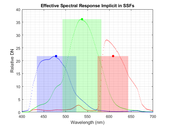
If we carry out the wavelength by wavelength multiplication with the components selected in the last article – after assuming unity electronic gain $g_{rgb}$ and scaling for convenience by $hc$ divided by mean wavelength – we obtain the shown system Spectral Sensitivity Functions, one curve each for the three types of $rgb$ color pixels in the CFA

spectral response — Figure 3. Spectral Sensitivity Functions obtained from the components described in the last article after assuming unity electronic system gain and scaling by a factor equal to hc/550. Fictitious – but could represent SSFs of a digital camera and lens from a decade or so ago.

The Units of Light

In photography we assume that an object at the scene reflects the illuminant towards the lens, producing a certain light intensity per unit area there – what is properly called radiance ( $L$ ). To obtain the absolute response of our imaging system to it, all we have to do is supply the lens with $L(\lambda)$ , the Spectral Power Distribution of the incoming light as a function of wavelength, for instance standard daylight illuminant $D50$ after reflection by an 18% gray card, in radiometric units of $W/sr/m^2/nm$ . For more detail on $L$ see the article on angles and Lambertian reflection.

Recall that $W$ is the symbol for watts, the units of power; $sr$ stands for steradians, the units of solid angles; $m$ and $nm$ for meters and nanometers, the units of distance. Watts are really shorthand for joules per second, with joules $J$ the units of energy and seconds $s$ the units of time.

Given such a spectral power distribution at the lens, after interacting with the Spectral Sensitivity Functions, the output of the imaging system will be proportional to relative quanta per watt per nm. Relative quanta could refer to a current, a number of photoelectrons, a voltage or Data Numbers depending on where one looks deep into the electronics of the camera.

Determining Absolute Energy Projected on a Pixel

So what light intensity will a pixel see when there is a spectral stimulus equal to $L(\lambda)$ at the entrance of the lens? Assuming conservation of energy/throughput, spectral radiance $L(\lambda)$ collected by the (arbitrarily large) entrance pupil of the lens will present itself at the exit pupil, minus spectral transmission losses. To determine the energy projected on the area of a single pixel in the center of the sensor by such radiance during Exposure all we have to do is follow its units: $W/sr/m^2/nm$ , aka $J/s/sr/m^2/nm$ .

Therefore back-to-front we need: the wavelength bandwidth of interest, the area of the pixel, the solid angle representing the field of view of the pixel, and the integration time. We normally know exposure time ( $t$ expressed in seconds), the area of the pixel ( $p^2$ with pixel pitch $p$ in meters) and the range of visible wavelengths that we are interested in (380-780nm expressed in meters). So all that is left to determine is the number of steradians in the solid angle formed by the lens and the, say central, pixel of the sensor.^[3]

How Many Steradians in a Typical Lens?

The solid angle is formed by the exit pupil of the lens on one side and the pixel at its vertex on the other. With small angles it can be approximated by a right circular cone, refer to cone Ω formed by the light green lines between the lens and the sensor in Figure 4.^[*] By approximate definition, the number of steradians is then given by the area of the base of the cone divided by its height squared. In other words, for a lens focused at infinity, with unity pupil magnification and small half opening angles $\theta'$ , divide the area of the exit pupil by focal length $f$ squared.

Figure 4. The cone Ω formed by the exit pupil of the lens and a pixel in the center of the sensing plane.

The area of a circular exit pupil of diameter $D$ is equal to $\pi(D/2)^2$ . Dividing that area by focal length squared, the appropriate solid angle can be expressed approximately as

(2) $\begin{equation*} \Omega \approx \frac{\pi D^2}{4 f^2} =\frac{\pi}{4N^2} \text{ steradians} \end{equation*}$

with $N=\frac{f}{D}$ the f-number of the lens. For well corrected lenses that are not focused at infinity and/or with pupil magnification other than unity^[4], the working f-number $N_w=\frac{1}{2sin\theta'}$ can be used instead of $N$ .^[5] For more detail on this see the article on pupils and apertures.

Energy Projected on Silicon

With the solid angle in hand, and assuming 100% effective microlenses, we now have all the information needed to calculate the energy projected onto the photoelectric area of a pixel during Exposure by a spectral radiance $L(\lambda)$ at the front of the lens – after it has gone through all the filtering components of the imaging system:

(3) $\begin{equation*} e_{rgb} \approx \frac{\pi p^2 t}{4N^2} \int_{380_{nm}}^{780_{nm}}L(\lambda)\odot F_{rgb}(\lambda) d\lambda \end{equation*}$

all symbols as explained earlier. The units of $e_{rgb}$ are joules per pixel ( $J/px$ ) when distance and time are expressed in meters and seconds respectively. The integral in Equation (3) simply indicates the area under the curve resulting from the relative element-wise product. It evaluates to the energy expected just above the active material in the sensor. Clearly the energy is different depending on whether a given pixel is under the $r$ , $g$ or $b$ CFA filter.

Counts in the Raw Data

After the impinging spectral energy $e_{rgb}$ is converted to quanta by the photoelectric effect in silicon with consequent loss of efficiency $QE(\lambda)$ – and subsequent counting by the camera’s downstream analog to digital electronics – we obtain the approximate absolute trichromatic $r_{_L}g_{_L}b_{_L}$ values that will be written to the raw file

(4) $\begin{equation*} r_{_L}g_{_L}b_{_L} \approx \frac{\pi p^2 t}{4N^2} \int_{380_{nm}}^{780_{nm}}L(\lambda)\odot SSF_{rgb}(\lambda) d\lambda \end{equation*}$

with $r_{_L}g_{_L}b_{_L}$ the digital value triplet in the raw data (in $DN$ ), subscript $_L$ indicating absolute correspondence to input spectral radiance $L(\lambda)$ in units of $W/sr/m^2/nm$ , $SSF_{rgb}$ per Equation (1) and all other variables as described earlier. The wavelength by wavelength product represents the change in the spectral composition of light as it progressed through the imaging system, while integration is the job that pixels perform during exposure. Together they formally represent a dot or inner product.

The units of Equation (4) are $DN$ per pixel as a function of the Spectral Power Distribution of input radiance $L(\lambda)$ , for the given camera and lens. The values therefore represent the intensity (measurable amount) of light from the scene as captured by the imaging system linearly in the raw data. This is why raw data values (but often also downstream) are usually referred to as pixel ‘intensity’ in image processing.

If we are mainly interested in studying the effects of changing spectral responses, we vary input radiance $L(\lambda)$ and $SSF_{rgb}(\lambda)$ only – while treating all other variables in front of the integral as constants. This is often what is done in practice, greatly simplifying relative calculations.

Why it Matters

So that’s how the energy in the spectral radiance $L(\lambda)$ arriving at the lens is converted to raw data $DN$ in absolute physical terms. It is useful to understand the various steps involved in the conversion because imaging is all about estimating $L(\lambda)$ on an ideal sensing plane starting from values $r_{_L}g_{_L}b_{_L}$ captured in the raw file.

Vice versa, with this linear framework we can model expected raw values $r_{_L}g_{_L}b_{_L}$ if we have estimates for radiance $L(\lambda)$ at the lens and the imaging system’s spectral response in the form of $SSF_{rgb}(\lambda)$ . This can be quite useful when characterizing the system as we will soon see.

However photographers typically only have trichromatic raw data in DN from a capture – while Color Science is based on spectral energy. The first small step in bridging that gap is the subject of the next article.

Appendix: Effective SSF Wavelengths and Bandwidths

Assuming spectrally flat radiance and going relative, we can ignore the constants in front of Equation (4) and proceed with the integral (in practice they are calculated by numerical sum). The SSFs in Figure 3 would then produce raw data in DN in proportion to the integral of (or the area under) each curve. The relative trichromatic values under equi-energy illuminant $S_e$ would be:

$r$ = 21.9 DN, $g$ = 36.1 DN, $b$ = 21.9 DN

which we will write in vector notation as follows

$rgb$ = [21.9 36.1 21.9] DN.

These correspond to the following white balance multipliers

$K{rgb}$ = [1.6484 1.0000 1.6484].

If we had to simplify things and suggest a single wavelength to which those results could be ascribed we could take the sum of each wavelength weighted by the relative $\bar{r}$ , $\bar{g}$ or $\bar{b}$ function divided by its sum over the spectrum. Such an effective wavelength would be equivalent to the center of mass of the curve:

(5) $\begin{equation*} \lambda_{EFF}_{rgb} = \frac{\int SSF_{rgb}(\lambda)\odot \lambda d\lambda}{\int SSF_{rgb}(\lambda) d\lambda} \end{equation*}$

For our example SSFs the effective wavelengths of $rgb$ pixels are respectively:

$\lambda_{EFF}_{rgb}$ = [608.7 537.9 478.8] nm.

The effective bandwidths can instead be calculated by normalizing the SSFs to their respective maxima and integrating the result

(6) $\begin{equation*} \Delta\lambda_{EFF}_{rgb} = \frac{\int SSF_{rgb}(\lambda) d\lambda} {max(SSF_{rgb}(\lambda))} \end{equation*}$

$\Delta\lambda_{EFF}_{rgb}$ = [70.4, 90.2nm, 91.0] nm.

Having done all that the effective Response of the Spectral Sensitivity Functions derived in the last article and depicted in Figure 3 can be represented as follows

Figure 4. Effective Spectral Response produced by the Spectral Sensitivity Functions in the imaging system described in the last article, assuming flat spectral radiance at the lens. All three functions were scaled by a common factor to make the green curve peak at 36.1DN.

Notes and References

_{1. There are few resources online for measured SSFs of digital cameras, none too current:

a) “Reference data set for camera spectral sensitivity estimation, Maryam Mohammadzadeh Darrodi, Graham Finlayson, Teresa Goodman and Michal Mackiewicz, Vol. 32, No. 3 / March 2015 / J. Opt. Soc. Am. A”. The relative data, the paper and additional information are available in this page.

b) Christian Mauer’s Thesis at the Department of Media and Phototechnology, University of Applied Sciences Cologne, which you can find here

c) Jun Jiang, Dengyu Liu, Jinwei Gu and Sabine Susstrunk. “What is the Space of Spectral Sensitivity Functions for Digital Color Cameras?“, IEEE Workshop on the Applications of Computer Vision (WACV), 2013.

2. This article explains how to convert radiometric to photometric units.

3. wikipedia page with further information on solid angles.

4. When pupil magnification p is not unity, focal length at infinity f is replaced by effective focal length pf, see for instance Equation 10 here.

5. When the lens is not focused at infinity working f-number is used instead. The definition of working f-number can be found here.

6. A good discussion of radiometric sensing in imaging is provided in “Remote Sensing, the Image Chain Approach, 2nd Edition, John R. Scott, RIT, Oxford University Press, 2007”.}

Strolls with my Dog