In this article we confirm quantitatively that getting the White Point, hence the White Balance, right is essential to obtaining natural tones out of our captures. How quickly do colors degrade if the estimated Correlated Color Temperature is off?

In this article we confirm quantitatively that getting the White Point, hence the White Balance, right is essential to obtaining natural tones out of our captures. How quickly do colors degrade if the estimated Correlated Color Temperature is off?
In this article I bring together qualitatively the main concepts discussed in the series and argue that in many (most) cases a photographer’s job in order to obtain natural looking tones in their work during raw conversion is to get the illuminant and relative white balance right – and to step away from any slider found in menus with the word ‘color’ in them.

If you are an outdoor photographer trying to get balanced greens under an overcast sky – or a portrait photographer after good skin tones – dialing in the appropriate scene, illuminant and white balance puts the camera/converter manufacturer’s color science to work and gets you most of the way there safely. Of course the judicious photographer always knew to do that – hopefully now with a better appreciation as for why.
As we have seen in the previous post, knowing the characteristics of light at the scene is critical to be able to determine the color transform that will allow captured raw data to be naturally displayed from an output color space like ubiquitous sRGB.
The light source Spectral Power Distribution (SPD) corresponds to a unique White Point, namely a set of coordinates in the  color space, obtained by multiplying wavelength-by-wavelength its SPD (the blue curve below) by the response of the retina of a typical viewer, otherwise known as the CIE Color Matching Functions of a Standard Observer (
 in the plot)

Adding (integrating) the three resulting curves we get three values that represent the illuminant’s coordinates in the color space. The White Point is obtained by dividing these coordinates by the  value to normalize it to 1.
For example a Standard Daylight Illuminant with a Correlated Color Temperature of 5300 kelvins has a White Point of[1]
 = [0.9593 1.0000 0.8833]
assuming CIE (2012) 2-deg XYZ “physiologically relevant” Color Matching Functions from cvrl.org. Continue reading White Point, CCT and Tint
Building on a preceeding article of this series, once demosaiced raw data from a Bayer Color Filter Array sensor represents the captured image as a set of triplets, corresponding to the estimated light intensity at a given pixel under each of the three spectral filters part of the CFA. The filters are band-pass and named for the representative peak wavelength that they let through, typically red, green, blue.
Since the resulting intensities are linearly independent they can form the basis of a 3D coordinate system, with each triplet representing a point within it. The system is bounded in the raw data by the extent of the Analog to Digital Converter, with all three channels spanning the same range, from Black Level with no light to clipping with maximum recordable light. Therefore it can be thought to represent a space in the form of a cube – or better, a parallelepiped – with the origin at [0,0,0] and the opposite vertex at the clipping value in Data Numbers, expressed as [1,1,1] once normalized.

The job of the color transform is to project demosaiced raw data  to a standard output
  color space designed for viewing. Such spaces have names like
  ,
,  or
or  . The output space can also be shown in 3D as a parallelepiped with the origin at [0,0,0] with no light and the opposite vertex at [1,1,1] with maximum displayable light. Continue reading Linear Color Transforms
In the previous article we determined that the three  values recorded in the raw data in the center of the image plane in units of Data Numbers per pixel – by a digital camera and lens as a function of absolute spectral radiance
  at the lens – can be estimated as follows:
(1) 
with subscript  indicating absolute-referred units and
  the three system Spectral Sensitivity Functions. In this series of articles
  is wavelength by wavelength multiplication (what happens to the spectrum of light as it progresses through the imaging system) and the integral just means the area under each of the three resulting curves (integration is what the pixels do during exposure). Together they represent an inner or dot product. All variables in front of the integral were previously described and can be considered constant for a given photographic setup. Continue reading Connecting Photographic Raw Data to Tristimulus Color Science
In the previous article we (I) learned that the Spectral Sensitivity Functions of a given digital camera and lens are the result of the interaction of light from the scene with all of the spectrally varied components that make up the imaging system: mainly the lens, ultraviolet/infrared hot mirror, Color Filter Array and other filters, finally the photoelectric layer of the sensor, which is normally silicon in consumer kit.

In this one we will put the process on a more formal theoretical footing, setting the stage for the next few on the role of white balance.
Photography works because visible light from one or more sources reaches the scene and is reflected in the direction of the camera, which then captures a signal proportional to it. The journey of light can be described in integrated units of power all the way to the sensor, for instance so many watts per square meter. However ever since Newton we have known that such total power is in fact the result of the weighted sum of contributions by every frequency that makes up the light, what he called its spectrum.
Our ability to see and record color depends on knowing the distribution of the power contained within a subset of these frequencies and how it interacts with the various objects in its path. This article is about how a typical digital camera for photographers interacts with the spectrum arriving from the scene: we will dissect what is sometimes referred to as the system’s Spectral Response or Sensitivity.

Canon recently introduced its EOS-1D X Mark III Digital Single-Lens Reflex [Edit: and now also possibly the R5 Mirrorless ILC] touting a new and improved Anti-Aliasing filter, which they call a High-Res Gaussian Distribution LPF, claiming that
“This not only helps to suppress moiré and color distortion,
but also improves resolution.”

In this article we will try to dissect the marketing speak and understand a bit better the theoretical implications of the new AA. For the abridged version, jump to the Conclusions at the bottom. In a picture:

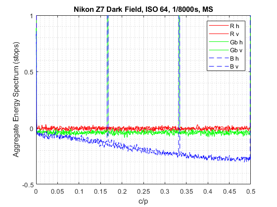
A spectrogram, also sometimes referred to as a periodogram, is a visual representation of the Power Spectrum of a signal. Power Spectrum answers the question “How much power is contained in the frequency components of the signal”. In digital photography a Power Spectrum can show the relative strength of repeating patterns in captures and whether processing has been applied.
In this article I will describe how you can construct a spectrogram and how to interpret it, using dark field raw images taken with the lens cap on as an example. This can tell us much about the performance of our imaging devices in the darkest shadows and how well tuned their sensors are there.
In this article we shall find that the effect of a Bayer CFA on the spatial frequencies and hence the ‘sharpness’ information captured by a sensor compared to those from the corresponding monochrome version can go from (almost) nothing to halving the potentially unaliased range – based on the chrominance content of the image and the direction in which the spatial frequencies are being stressed. Continue reading Bayer CFA Effect on Sharpness
Now that we know how to create a 3×3 linear matrix to convert white balanced and demosaiced raw data into  connection space – and where to obtain the 3×3 linear matrix to then convert it to a standard output color space like sRGB – we can take a closer look at the matrices and apply them to a real world capture chosen for its wide range of chromaticities.

We understand from the previous article that rendering color with Adobe DNG raw conversion essentially means mapping raw data in the form of triplets into a standard color space via a Profile Connection Space in a two step process
![\[ Raw Data \rightarrow XYZ_{D50} \rightarrow RGB_{standard} \]](https://i0.wp.com/www.strollswithmydog.com/wordpress/wp-content/ql-cache/quicklatex.com-164bf80016fc459bad893b6930883830_l3.png?resize=298%2C15&ssl=1 "Rendered by QuickLaTeX.com")
The first step white balances and demosaics the raw data, which at that stage we will refer to as , followed by converting it to Profile Connection Space through linear projection by an unknown ‘Forward Matrix’ (as DNG calls it) of the form
(1) ![\begin{equation*} \left[ \begin{array}{c} X_{D50} \\ Y_{D50} \\ Z_{D50} \end{array} \right] = \begin{bmatrix} a_{11} & a_{12} & a_{13} \\ a_{21} & a_{22} & a_{23} \\ a_{31} & a_{32} & a_{33} \end{bmatrix} \left[ \begin{array}{c} r \\ g \\ b \end{array} \right] \end{equation*}](https://i0.wp.com/www.strollswithmydog.com/wordpress/wp-content/ql-cache/quicklatex.com-f4f3535c40e6f7d83ee139eaf9633956_l3.png?resize=273%2C64&ssl=1 "Rendered by QuickLaTeX.com")
with data as column-vectors in a 3xN array. Determining the nine  coefficients of this matrix
  is the main subject of this article[1]. Continue reading Color: Determining a Forward Matrix for Your Camera
How do we translate captured image information into a stimulus that will produce the appropriate perception of color? It’s actually not that complicated[1].
Recall from the introductory article that a photon absorbed by a cone type ( ,
,  or
or  ) in the fovea produces the same stimulus to the brain regardless of its wavelength[2]. Take the example of the eye of an observer which focuses on the retina the image of a uniform object with a spectral photon distribution of 1000 photons/nm in the 400 to 720nm wavelength range and no photons outside of it.
Because the system is linear, cones in the foveola will weigh the incoming photons by their relative sensitivity (probability) functions and add the result up to produce a stimulus proportional to the area under the curves. For instance a cone may see about 321,000 photons arrive and produce a relative stimulus of about 94,700, the weighted area under the curve:

This article will set the stage for a discussion on how pleasing color is produced during raw conversion. The easiest way to understand how a camera captures and processes ‘color’ is to start with an example of how the human visual system does it.
Light from the sun strikes leaves on a tree. The foliage of the tree absorbs some of the light and reflects the rest diffusely towards the eye of a human observer. The eye focuses the image of the foliage onto the retina at its back. Near the center of the retina there is a small circular area called fovea centralis which is dense with light receptors of well defined spectral sensitivities called cones. Information from the cones is pre-processed by neurons and carried by nerve fibers via the optic nerve to the brain where, after some additional psychovisual processing, we recognize the color of the foliage as green[1].

Continue reading An Introduction to Color in Digital Cameras
Several sites for photographers perform spatial resolution ‘sharpness’ testing of a specific lens and digital camera set up by capturing a target. You can also measure your own equipment relatively easily to determine how sharp your hardware is. However comparing results from site to site and to your own can be difficult and/or misleading, starting from the multiplicity of units used: cycles/pixel, line pairs/mm, line widths/picture height, line pairs/image height, cycles/picture height etc.
This post will address the units involved in spatial resolution measurement using as an example readings from the popular slanted edge method, although their applicability is generic.
My preferred method for measuring the spatial resolution performance of photographic equipment these days is the slanted edge method. It requires a minimum amount of additional effort compared to capturing and simply eye-balling a pinch, Siemens or other chart but it gives more, useful, accurate, quantitative information in the language and units that have been used to characterize optical systems for over a century: it produces a good approximation to the Modulation Transfer Function of the two dimensional camera/lens system impulse response – at the location of the edge in the direction perpendicular to it.
Much of what there is to know about an imaging system’s spatial resolution performance can be deduced by analyzing its MTF curve, which represents the system’s ability to capture increasingly fine detail from the scene, starting from perceptually relevant metrics like MTF50, discussed a while back.
In fact the area under the curve weighted by some approximation of the Contrast Sensitivity Function of the Human Visual System is the basis for many other, better accepted single figure ‘sharpness‘ metrics with names like Subjective Quality Factor (SQF), Square Root Integral (SQRI), CMT Acutance, etc. And all this simply from capturing the image of a slanted edge in a raw file, which one can actually and somewhat easily do at home, as presented in the next article.