Canon recently introduced its EOS-1D X Mark III Digital Single-Lens Reflex [Edit: and now also possibly the R5 Mirrorless ILC] touting a new and improved Anti-Aliasing filter, which they call a High-Res Gaussian Distribution LPF, claiming that
“This not only helps to suppress moiré and color distortion, but also improves resolution.”
Figure 1. Artist’s rendition of new High-res Low Pass Filter, courtesy of Canon USA
In this article we will try to dissect the marketing speak and understand a bit better the theoretical implications of the new AA. For the abridged version, jump to the Conclusions at the bottom. In a picture:
Now that we know how to create a 3×3 linear matrix to convert white balanced and demosaiced raw data into connection space – and where to obtain the 3×3 linear matrix to then convert it to a standard output color space like sRGB – we can take a closer look at the matrices and apply them to a real world capture chosen for its wide range of chromaticities.
Figure 1. Image with color converted using the forward linear matrix discussed in the article.
We understand from the previous article that rendering color with Adobe DNG raw conversion essentially means mapping raw data in the form of triplets into a standard color space via a Profile Connection Space in a two step process
The first step white balances and demosaics the raw data, which at that stage we will refer to as , followed by converting it to Profile Connection Space through linear projection by an unknown ‘Forward Matrix’ (as DNG calls it) of the form
How do we translate captured image information into a stimulus that will produce the appropriate perception of color? It’s actually not that complicated[1].
Recall from the introductory article that a photon absorbed by a cone type (, or ) in the fovea produces the same stimulus to the brain regardless of its wavelength[2]. Take the example of the eye of an observer which focuses on the retina the image of a uniform object with a spectral photon distribution of 1000 photons/nm in the 400 to 720nm wavelength range and no photons outside of it.
Because the system is linear, cones in the foveola will weigh the incoming photons by their relative sensitivity (probability) functions and add the result up to produce a stimulus proportional to the area under the curves. For instance a cone may see about 321,000 photons arrive and produce a relative stimulus of about 94,700, the weighted area under the curve:
Figure 1. Light made up of 321k photons of broad spectrum and constant Spectral Photon Distribution between 400 and 720nm is weighted by cone sensitivity to produce a relative stimulus equivalent to 94,700 photons, proportional to the area under the curve
This article will set the stage for a discussion on how pleasing color is produced during raw conversion. The easiest way to understand how a camera captures and processes ‘color’ is to start with an example of how the human visual system does it.
An Example: Green
Light from the sun strikes leaves on a tree. The foliage of the tree absorbs some of the light and reflects the rest diffusely towards the eye of a human observer. The eye focuses the image of the foliage onto the retina at its back. Near the center of the retina there is a small circular area called fovea centralis which is dense with light receptors of well defined spectral sensitivities called cones. Information from the cones is pre-processed by neurons and carried by nerve fibers via the optic nerve to the brain where, after some additional psychovisual processing, we recognize the color of the foliage as green[1].
Figure 1. The human eye absorbs light from an illuminant reflected diffusely by the object it is looking at.
What are the basic low level steps involved in raw file conversion? In this article I will discuss what happens under the hood of digital camera raw converters in order to turn raw file data into a viewable image, a process sometimes referred to as ‘rendering’. We will use the following raw capture by a Nikon D610 to show how image information is transformed at every step along the way:
Figure 1. Nikon D610 with AF-S 24-120mm f/4 lens at 24mm f/8 ISO100, minimally rendered from raw by Octave/Matlab following the steps outlined in the article.
This post will continue looking at the spatial frequency response measured by MTF Mapper off slanted edges in DPReview.com raw captures and relative fits by the ‘sharpness’ model discussed in the last few articles. The model takes the physical parameters of the digital camera and lens as inputs and produces theoretical directional system MTF curves comparable to measured data. As we will see the model seems to be able to simulate these systems well – at least within this limited set of parameters.
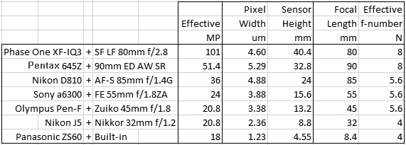
The following fits refer to the green channel of a number of interchangeable lens digital camera systems with different lenses, pixel sizes and formats – from the current Medium Format 100MP champ to the 1/2.3″ 18MP sensor size also sometimes found in the best smartphones. Here is the roster with the cameras as set up:
The series of articles starting here outlines a model of how the various physical components of a digital camera and lens can affect the ‘sharpness’ – that is the spatial resolution – of the images captured in the raw data. In this one we will pit the model against MTF curves obtained through the slanted edge method[1]from real world raw captures both with and without an anti-aliasing filter.
With a few simplifying assumptions, which include ignoring aliasing and phase, the spatial frequency response (SFR or MTF) of a photographic digital imaging system near the center can be expressed as the product of the Modulation Transfer Function of each component in it. For a current digital camera these would typically be the main ones:
We now know how to calculate the two dimensional Modulation Transfer Function of a perfect lens affected by diffraction, defocus and third order Spherical Aberration – under monochromatic light at the given wavelength and f-number. In digital photography however we almost never deal with light of a single wavelength. So what effect does an illuminant with a wide spectral power distribution, going through the color filter of a typical digital camera CFA before the sensor have on the spatial frequency responses discussed thus far?
Spherical Aberration (SA) is one key component missing from our MTF toolkit for modeling an ideal imaging system’s ‘sharpness’ in the center of the field of view in the frequency domain. In this article formulas will be presented to compute the two dimensional Point Spread and Modulation Transfer Functions of the combination of diffraction, defocus and third order Spherical Aberration for an otherwise perfect lens with a circular aperture.
Spherical Aberrations result because most photographic lenses are designed with quasi spherical surfaces that do not necessarily behave ideally in all situations. For instance, they may focus light on systematically different planes depending on whether the respective ray goes through the exit pupil closer or farther from the optical axis, as shown below:
Figure 1. Top: an ideal spherical lens focuses all rays on the same focal point. Bottom: a practical lens with Spherical Aberration focuses rays that go through the exit pupil based on their radial distance from the optical axis. Image courtesy Andrei Stroe.
This series of articles has dealt with modeling an ideal imaging system’s ‘sharpness’ in the frequency domain. We looked at the effects of the hardware on spatial resolution: diffraction, sampling interval, sampling aperture (e.g. a squarish pixel), anti-aliasing OLPAF filters. The next two posts will deal with modeling typical simple imperfections related to the lens: defocus and spherical aberrations.
Defocus = OOF
Defocus means that the sensing plane is not exactly where it needs to be for image formation in our ideal imaging system: the image is therefore out of focus (OOF). Said another way, light from a point source would go through the lens but converge either behind or in front of the sensing plane, as shown in the following diagram, for a lens with a circular aperture:
Figure 1. Top to bottom: Back Focus, In Focus, Front Focus. To the right is how the relative PSF would look like on the sensing plane. Image under license courtesy of Brion.
This article is part of a continuing series on the determinants of sharpness in an imaging system and will discuss a simple frequency domain model for an AntiAliasing (or Optical Low Pass) Filter, a hardware component sometimes found in a digital imaging system[1]. The filter typically sits just above the sensor and its objective is to block as much of the aliasing and moiré creating energy above the monochrome Nyquist spatial frequency while letting through as much as possible of the real image forming energy below that, hence the low-pass designation.
Figure 1. The blue line indicates the pass through performance of an ideal anti-aliasing filter presented with an Airy PSF (Original): pass all spatial frequencies below Nyquist (0.5 c/p) and none above that. No filter has such ideal characteristics and if it did its hard edges would result in undesirable ringing in the image.
In consumer digital cameras it is often implemented by introducing one or two birefringent plates in the sensor’s filter stack. This is how Nikon shows it for one of its DSLRs:
Figure 2. Typical Optical Low Pass Filter implementation in a current Digital Camera, courtesy of Nikon USA (yellow displacement ‘d’ added).
Having shown that our simple two dimensional MTF model is able to predict the performance of the combination of a perfect lens and square monochrome pixel with 100% Fill Factor we now turn to the effect of the sampling interval on spatial resolution according to the guiding formula:
(1)
The hats in this case mean the Fourier Transform of the relative component normalized to 1 at the origin (), that is the individual MTFs of the perfect lens PSF, the perfect square pixel and the delta grid; represents two dimensional convolution.
Sampling in the Spatial Domain
While exposed a pixel sees the scene through its aperture and accumulates energy as photons arrive. Below left is the representation of, say, the intensity that a star projects on the sensing plane, in this case resulting in an Airy pattern since we said that the lens is perfect. During exposure each pixel integrates (counts) the arriving photons, an operation that mathematically can be expressed as the convolution of the shown Airy pattern with a square, the size of effective pixel aperture, here assumed to have 100% Fill Factor. It is the convolution in the continuous spatial domain of lens PSF with pixel aperture PSF shown in Equation (2) of the first article in the series.
Sampling is then the product of an infinitesimally small Dirac delta function at the center of each pixel, the red dots below left, by the result of the convolution, producing the sampled image below right.
Figure 1. Left, 1a: A highly zoomed (3200%) image of the lens PSF, an Airy pattern, projected onto the imaging plane where the sensor sits. Pixels shown outlined in yellow. A red dot marks the sampling coordinates. Right, 1b: The sampled image zoomed at 16000%, 5x as much, because in this example each pixel’s width is 5 linear units on the side.
Now that we know from the introductory article that the spatial frequency response of a typical perfect digital camera and lens (its Modulation Transfer Function) can be modeled simply as the product of the Fourier Transform of the Point Spread Function of the lens and pixel aperture, convolved with a Dirac delta grid at cycles-per-pixel pitch spacing
This article is a little esoteric so one may want to skip it unless one is interested in the underlying mechanisms that cause quantization error as photographic signal and noise approach the darkest levels of acceptable dynamic range in our digital cameras: one least significant bit in the raw data. We will use our simplified camera model and deal with Poissonian Signal and Gaussian Read Noise separately – then attempt to bring them together.
Physicists and mathematicians over the last few centuries have spent a lot of their time studying light and electrons, the key ingredients of digital photography. In so doing they have left us with a wealth of theories to explain their behavior in nature and in our equipment. In this article I will describe how to simulate the information generated by a uniformly illuminated imaging system using open source Octave (or equivalently Matlab) utilizing some of these theories.
Since as you will see the simulations are incredibly (to me) accurate, understanding how the simulator works goes a long way in explaining the inner workings of a digital sensor at its lowest levels; and simulated data can be used to further our understanding of photographic science without having to run down the shutter count of our favorite SLRs. This approach is usually referred to as Monte Carlo simulation.
Whether the human visual system perceives a displayed slow changing gradient of tones, such as a vast expanse of sky, as smooth or posterized depends mainly on two well known variables: the Weber-Fechner Fraction of the ‘steps’ in the reflected/produced light intensity (the subject of this article); and spatial dithering of the light intensity as a result of noise (the subject of a future one).
We’ve seen how information about a photographic scene is collected in the ISOless/invariant range of a digital camera sensor, amplified, converted to digital data and stored in a raw file. For a given Exposure the best information quality (IQ) about the scene is available right at the photosites, only possibly degrading from there – but a properly designed** fully ISO invariant imaging system is able to store it in its entirety in the raw data. It is able to do so because the information carrying capacity (photographers would call it the dynamic range) of each subsequent stage is equal to or larger than the previous one. Cameras that are considered to be (almost) ISOless from base ISO include the Nikon D7000, D7200 and the Pentax K5. All digital cameras become ISO invariant above a certain ISO, the exact value determined by design compromises.
Figure 1: Simplified Scene Information Transfer in an ISO Invariant Imaging System at base ISO
In this article we’ll look at a class of imagers that are not able to store the whole information available at the photosites in one go in the raw file for a substantial portion of their working ISOs. The photographer can in such a case choose out of the full information available at the photosites what smaller subset of it to store in the raw data by the selection of different in-camera ISOs. Such cameras are sometimes improperly referred to as ISOful. Most Canon DSLRs fall into this category today. As do kings of darkness such as the Sony a7S or Nikon D5.
In the last few posts I have made the case that Image Quality in a digital camera is entirely dependent on the light Information collected at a sensor’s photosites during Exposure. Any subsequent processing – whether analog amplification and conversion to digital in-camera and/or further processing in-computer – effectively applies a set of Information Transfer Functions to the signal that when multiplied together result in the data from which the final photograph is produced. Each step of the way can at best maintain the original Information Quality (IQ) but in most cases it will degrade it somewhat.
IQ: Only as Good as at Photosites’ Output
This point is key: in a well designed imaging system** the final image IQ is only as good as the scene information collected at the sensor’s photosites, independently of how this information is stored in the working data along the processing chain, on its way to being transformed into a pleasing photograph. As long as scene information is properly encoded by the system early on, before being written to the raw file – and information transfer is maintained in the data throughout the imaging and processing chain – final photograph IQ will be virtually the same independently of how its data’s histogram looks along the way.
We know that the best Information Quality possible collected from the scene by a digital camera is available right at the output of the sensor and it will only be degraded from there. This article will discuss what happens to this information as it is transferred through the imaging system and stored in the raw data. It will use the simple language outlined in the last post to explain how and why the strategy for Capturing the best Information or Image Quality (IQ) possible from the scene in the raw data involves only two simple steps:
1) Maximizing the collected Signal given artistic and technical constraints; and
2) Choosing what part of the Signal to store in the raw data and what part to leave behind.
The second step is only necessary if your camera is incapable of storing the entire Signal at once (that is it is not ISO invariant) and will be discussed in a future article. In this post we will assume an ISOless imaging system.
My camera has an engineering Dynamic Range of 14 stops, how many bits do I need to encode that DR? Well, to encode the whole Dynamic Range 1 bit could suffice, depending on the content and the application. The reason is simple, dynamic range is only concerned with the extremes, not with tones in between:
So in theory we only need 1 bit to encode it: zero for minimum signal and one for maximum signal, like so
Dynamic Range (DR) in Photography usually refers to the linear working signal range, from darkest to brightest, that the imaging system is capable of capturing and/or displaying. It is expressed as a ratio, in stops:
It is a key Image Quality metric because photography is all about contrast, and dynamic range limits the range of recordable/ displayable tones. Different components in the imaging system have different working dynamic ranges and the system DR is equal to the dynamic range of the weakest performer in the chain.
Imperfections in an imaging system’s capture process manifest themselves in the form of deviations from the expected signal. We call these imperfections ‘noise’ because they introduce grain and artifacts in our images. The fewer the imperfections, the lower the noise, the higher the image quality.
However, because the Human Visual System is adaptive within its working range, it’s not the absolute amount of noise that matters to perceived Image Quality (IQ) as much as the amount of noise relative to the signal – represented for instance by the Signal to Noise Ratio (SNR). That’s why to characterize the performance of a sensor in addition to signal and noise we also need to determine its sensitivity and the maximum signal it can detect.
In this series of articles I will describe how to use the Photon Transfer method and a spreadsheet to determine basic IQ performance metrics of a digital camera sensor. It is pretty easy if we keep in mind the simple model of how light information is converted into raw data by digital cameras:
Olympus just announced the E-M5 Mark II, an updated version of its popular micro Four Thirds E-M5 model, with an interesting new feature: its 16MegaPixel sensor, presumably similar to the one in other E-Mx bodies, has a high resolution mode where it gets shifted around by the image stabilization servos during exposure to capture, as they say in their press release
‘resolution that goes beyond full-frame DSLR cameras. 8 images are captured with 16-megapixel image information while moving the sensor by 0.5 pixel steps between each shot. The data from the 8 shots are then combined to produce a single, super-high resolution image, equivalent to the one captured with a 40-megapixel image sensor.’
A great idea that could give a welcome boost to the ‘sharpness’ of this handy system. Preliminary tests show that the E-M5 mk II 64MP High-Res mode gives some advantage in MTF50 linear spatial resolution compared to the Standard Shot 16MP mode with the captures in this post. Plus it apparently virtually eliminates the possibility of aliasing and moiré. Great stuff, Olympus.
Equivalence – as we’ve discussed one of the fairest ways to compare the performance of two cameras of different physical formats, characteristics and specifications – essentially boils down to two simple realizations for digital photographers:
metrics need to be expressed in units of picture height (or diagonal where the aspect ratio is significantly different) in order to easily compare performance with images displayed at the same size; and
focal length changes proportionally to sensor size in order to capture identical scene content on a given sensor, all other things being equal.
The first realization should be intuitive (see next post). The second one is the subject of this post: I will deal with it through a couple of geometrical diagrams.
Determining the Signal to Noise Ratio (SNR) curves of your digital camera at various ISOs and extracting from them the underlying IQ metrics of its sensor can help answer a number of questions useful to photography. For instance whether/when to raise ISO; what its dynamic range is; how noisy its output could be in various conditions; or how well it is likely to perform compared to other Digital Still Cameras. As it turns out obtaining the relative data is a little time consuming but not that hard. All you need is your camera, a suitable target, a neutral density filter, dcraw or libraw or similar software to access the linear raw data – and a spreadsheet.
In photography the higher the ratio of Signal to Noise, the less grainy the final image normally looks. The Signal-to-Noise-ratio SNR is therefore a key component of Image Quality. Let’s take a closer look at it. Continue reading SNR Curves and IQ in Digital Cameras→
Effective Quantum Efficiency as I calculate it is an estimate of the probability that a visible photon – from a ‘Daylight’ blackbody radiating source at a temperature of 5300K impinging on the sensor in question after making it through its IR filter, UV filter, AA low pass filter, microlenses, average Color Filter – will produce a photoelectron upon hitting silicon:
One of the fairest ways to compare the performance of two cameras of different physical characteristics and specifications is to ask a simple question: which photograph would look better if the cameras were set up side by side, captured identical scene content and their output were then displayed and viewed at the same size?
Achieving this set up and answering the question is anything but intuitive because many of the variables involved, like depth of field and sensor size, are not those we are used to dealing with when taking photographs. In this post I would like to attack this problem by first estimating the output signal of different cameras when set up to capture Equivalent images.
It’s a bit long so I will give you the punch line first: digital cameras of the same generation set up equivalently will typically generate more or less the same signal in independently of format. Ignoring noise, lenses and aspect ratio for a moment and assuming the same camera gain and number of pixels, they will produce identical raw files. Continue reading Equivalence and Equivalent Image Quality: Signal→
You want to measure how sharp your camera/lens combination is to make sure it lives up to its specs. Or perhaps you’d like to compare how well one lens captures spatial resolution compared to another you own. Or perhaps again you are in the market for new equipment and would like to know what could be expected from the shortlist. Or an old faithful is not looking right and you’d like to check it out. So you decide to do some testing. Where to start?
In the next four articles I will walk you through my methodology based on captures of slanted edge targets:
How many visible photons hit a pixel on my sensor? The answer depends on Exposure, Spectral power distribution of the arriving light and effective pixel area. With a few simplifying assumptions it is not difficult to calculate that with a typical Daylight illuminant the number is roughly 11,760 photons per lx-s per . Without the simplifying assumptions* it reduces to about 11,000. Continue reading How Many Photons on a Pixel→
I measured the Spectral Photon Distribution of the three CFA filters of a Nikon D610 in ‘Daylight’ conditions with a cheap spectrometer. Taking a cue from this post I pointed it at light from the sun reflected off a gray card and took a raw capture of the spectrum it produced.
An ImageJ plot did the rest. I took a dozen captures at slightly different angles to catch the picture of the clearest spectrum. Shown are the three spectral curves averaged over the two best opposing captures, each proportional to the number of photons let through by the respective Color Filter. The units on the vertical axis are raw black-subtracted values from the raw file (DN), therefore the units on the vertical axis are proportional to the number of incident photons in each case. The Photopic Eye Luminous Efficiency Function (2 degree, Sharpe et al 2005) is also shown for reference, scaled to the same maximum as the green curve (although in energy units, my bad). Continue reading Nikon CFA Spectral Power Distribution→
Is MTF50 a good proxy for perceived sharpness? In this article and those that follow MTF50 indicates the spatial frequency at which the Modulation Transfer Function of an imaging system is half (50%) of what it would be if the system did not degrade detail in the image painted by incoming light.
It makes intuitive sense that the spatial frequencies that are most closely related to our perception of sharpness vary with the size and viewing distance of the displayed image.
For instance if an image captured by a Full Frame camera is viewed at ‘standard’ distance (that is a distance equal to its diagonal), it turns out that the portion of the MTF curve most representative of perceived sharpness appears to be around MTF90. On the other hand, when pixel peeping the spatial frequencies around MTF50 look to be a decent, simple to calculate indicator of it, assuming a well set up imaging system in good working conditions. Continue reading MTF50 and Perceived Sharpness→


 connection space – and where to obtain the 3×3 linear matrix to then convert it to a standard output color space like sRGB – we can take a closer look at the matrices and apply them to a real world capture chosen for its wide range of chromaticities.
 triplets into a standard color space via a Profile Connection Space in a two step process
![\[ Raw Data \rightarrow XYZ_{D50} \rightarrow RGB_{standard} \]](https://i0.wp.com/www.strollswithmydog.com/wordpress/wp-content/ql-cache/quicklatex.com-164bf80016fc459bad893b6930883830_l3.png?resize=298%2C15&ssl=1 "Rendered by QuickLaTeX.com")
![\begin{equation*} \left[ \begin{array}{c} X_{D50} \\ Y_{D50} \\ Z_{D50} \end{array} \right] = \begin{bmatrix} a_{11} & a_{12} & a_{13} \\ a_{21} & a_{22} & a_{23} \\ a_{31} & a_{32} & a_{33} \end{bmatrix} \left[ \begin{array}{c} r \\ g \\ b \end{array} \right] \end{equation*}](https://i0.wp.com/www.strollswithmydog.com/wordpress/wp-content/ql-cache/quicklatex.com-f4f3535c40e6f7d83ee139eaf9633956_l3.png?resize=273%2C64&ssl=1 "Rendered by QuickLaTeX.com")
 coefficients of this matrix
  is the main subject of this article
 ,
,  or
or  ) in the fovea produces the same stimulus to the brain regardless of its wavelength


 ), that is the individual MTFs of the perfect lens PSF, the perfect square pixel and the delta grid;
  represents two dimensional convolution.

 here indicating normalization to one at the origin). I used Matlab to generate the examples below but you can easily do the same with a spreadsheet.
![\[ DR = \frac{Maximum Signal}{Minimum Signal} \]](https://i0.wp.com/www.strollswithmydog.com/wordpress/wp-content/ql-cache/quicklatex.com-0ef4805cfe0248405c147608a20bbc30_l3.png?resize=194%2C40&ssl=1 "Rendered by QuickLaTeX.com")
![\[ DR = log_2(\frac{Maximum Acceptable Signal}{Minimum Acceptable Signal}) \]](https://i0.wp.com/www.strollswithmydog.com/wordpress/wp-content/ql-cache/quicklatex.com-90d22584b8704a2407dc7c112466d0a6_l3.png?resize=321%2C41&ssl=1 "Rendered by QuickLaTeX.com")


 the signal in photoelectrons and
  the
the  independently of format. Ignoring noise, lenses and aspect ratio for a moment and assuming the same camera gain and number of pixels, they will produce identical raw files.
  .
. 