One of the fairest ways to compare the performance of two cameras of different physical characteristics and specifications is to ask a simple question: which photograph would look better if the cameras were set up side by side, captured identical scene content and their output were then displayed and viewed at the same size?

Achieving this set up and answering the question is anything but intuitive because many of the variables involved, like depth of field and sensor size, are not those we are used to dealing with when taking photographs.  In this post I would like to attack this problem by first estimating the output signal of different cameras when set up to capture Equivalent images.

It’s a bit long so I will give you the punch line first:  digital cameras of the same generation set up equivalently will typically generate more or less the same signal in independently of format.  Ignoring noise, lenses and aspect ratio for a moment and assuming the same camera gain and number of pixels, they will produce identical raw files.

Final displayed images are defined as Equivalent for the purpose of this post if and only if:

• They measure the same length diagonally (same display size)
• They are viewed from the same distance by a person of average visual acuity (same Circle of Confusion)
• They represent exactly the same scene (same lighting, subject and field of view)
• The perspective in the captured scene is the same (same distance to subject)
• They are subject to the same motion blur constraints (same exposure time)
• They show the same depth of field (DOF)

Given all that the first step is realizing that the signal, that is the total mean number of photoelectrons () produced by a uniformly illuminated sensor, is equal to

(1)  

where
is Luminance from the scene in cd/m
t is exposure time in seconds
eQE is the effective Quantum Efficiency of the sensor
N is the f-number at the time of exposure
is the sensing area in square microns
is an illuminant and lens dependent constant (see the figure below for its definition)

as discussed earlier.   If is the area of a pixel the mean raw value corresponding to this signal recorded by the camera in the raw file is simply  times a constant gain, which is controlled by the in-camera ISO setting:

To express this signal in Equivalent photographic terms we need formulas for depth of field (DOF), the diameter of the circle of confusion (C) and field of view (FOV).  Here they are, with a few simplifying assumptions:

(2)  

where is the f-number, is the distance from the camera to the subject in-focus plane and is focal length, all in meters.  The typically valid simplifying assumption here is that the circle of confusion (C) on the sensor is small compared to aperture:

(3)  

where is the length of the sensor diagonal and 50 cycles per degree on the retina is maximum average human acuity.  The simplifying assumption here is that the final photographs are viewed at a standard distance equal to the length of their diagonal.

Finally, we can write the following relationship to take into consideration the diagonal FOV as seen from the sensor:

(4)  

where is the conjugate in object space of the sensor’s diagonal (refer to the figure above).

Plugging (3) and (4) into (2) and solving for N we get

   

which together with rewriting the area of the sensor in terms of its diagonal

   

– with the aspect ratio of the sensor (e.g. 4:3) – we can then substitute into (1) to obtain the total mean signal in out of the given sensor in terms of the variables of Equivalence:

(5)  

If you are interested in the signal output by the average pixel, simply divide (5) by the number of pixels in the sensor.  Multiplying that by camera gain will yield the mean raw value written to the file in ADU.

The formula looks complex.  However, in an Equivalent situation many of these variables are shared constants for the differing cameras. For instance scene Luminance, exposure time, DOF and the field of view diagonal .   Collecting all common constants into , including the lens and illuminant specific factors present in , we obtain the Equivalent Total Signal formula:

(6)  

In other words – other than for their lenses (), aspect ratio () and effective quantum efficiency () – in an Equivalent situation the total signal in photoelectrons out of different sensors is exactly the same independently of format size.

Dividing (6) by the number of pixels in a sensor results in the Equivalent Signal produced by the average pixel:

(7)  

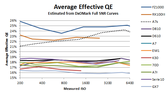
In practice differences in aspect ratio and effective Quantum Efficiency eQE are often quite limited, especially if viewed in stops.  For instance the fraction above reduces to 0.462 for an APS-C or 135 Full Frame format, 0.480 for Four Thirds, and 0.488 for 8×10.   One must take a little more care with eQE values even though they are typically within 10-15% of each other within a sensor generation fabbed with similar technology.  New technologies like BSI (seen below in the FZ1000 and RX100III curves) can on the other hand have quite an impact.

Ignoring noise and lenses and assuming the same aspect ratio, number of pixels, eQE and camera gain, cameras set up to record Equivalent captures will produce identical raw files independently of format and pixel size.

In a  future post we will discuss noise and Equivalence from a landscaper’s perspective.