Now that we know how to open 12-bit raw files captured with the new Raspberry Pi High Quality Camera, we can learn a bit more about the capabilities of its 1/2.3″ Sony IMX477 sensor from a keen photographer’s perspective. The subject is a bit dry, so I will give you the summary upfront. These figures were obtained with my HQ module at room temperature and the raspistill – -raw (-r) command:
| Raspberry Pi HQ Camera | raspistill --raw -ag 1 | Comments |
|---|---|---|
| Black Level | 256.3 DN | 256.0 - 257.3 based on gain |
| White Level | 4095 | Constant throughout |
| Analog Gain | 1 | Gain Range 1 - 16 |
| Read Noise | 3 e-, gain 1 1.5 e-, gain 16 | 1.53 DN from black frame 11.50 DN |
| Clipping (FWC) | 8180 e- | at base gain, 3400e-/um^2 |
| Dynamic Range | 11.15 stops 11.3 stops | SNR = 1 to Clipping Read Noise to Clipping |
| System Gain | 0.47 DN/e- | at base analog gain |
| Star Eater Algorithm | Partly Defeatable | All channels - from base gain and from min shutter speed |
| Low Pass Filter | Yes | All channels - from base gain and from min shutter speed |

 connection space – and where to obtain the 3×3 linear matrix to then convert it to a standard output color space like sRGB – we can take a closer look at the matrices and apply them to a real world capture chosen for its wide range of chromaticities.
 triplets into a standard color space via a Profile Connection Space in a two step process
![\[ Raw Data \rightarrow XYZ_{D50} \rightarrow RGB_{standard} \]](https://i0.wp.com/www.strollswithmydog.com/wordpress/wp-content/ql-cache/quicklatex.com-164bf80016fc459bad893b6930883830_l3.png?resize=298%2C15&ssl=1 "Rendered by QuickLaTeX.com")
![\begin{equation*} \left[ \begin{array}{c} X_{D50} \\ Y_{D50} \\ Z_{D50} \end{array} \right] = \begin{bmatrix} a_{11} & a_{12} & a_{13} \\ a_{21} & a_{22} & a_{23} \\ a_{31} & a_{32} & a_{33} \end{bmatrix} \left[ \begin{array}{c} r \\ g \\ b \end{array} \right] \end{equation*}](https://i0.wp.com/www.strollswithmydog.com/wordpress/wp-content/ql-cache/quicklatex.com-f4f3535c40e6f7d83ee139eaf9633956_l3.png?resize=273%2C64&ssl=1 "Rendered by QuickLaTeX.com")
 coefficients of this matrix
  is the main subject of this article
 ,
,  or
or  ) in the fovea produces the same stimulus to the brain regardless of its wavelength


 here indicating normalization to one at the origin). I used Matlab to generate the examples below but you can easily do the same with a spreadsheet.
  ) that reflects the mix of spectral information captured in the raw data, divorced from downstream color science; and
 ) that reflects the luminance channel of the image as neutrally displayed, hence may be more perceptually relevant.


 the signal in photoelectrons and
  the
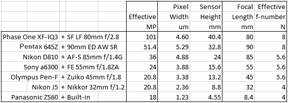
the  independently of format. Ignoring noise, lenses and aspect ratio for a moment and assuming the same camera gain and number of pixels, they will produce identical raw files.