nyquist | Strolls with my Dog

This post will continue looking at the spatial frequency response measured by MTF Mapper off slanted edges in DPReview.com raw captures and relative fits by the ‘sharpness’ model discussed in the last few articles. The model takes the physical parameters of the digital camera and lens as inputs and produces theoretical directional system MTF curves comparable to measured data. As we will see the model seems to be able to simulate these systems well – at least within this limited set of parameters.

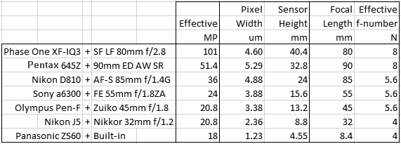
The following fits refer to the green channel of a number of interchangeable lens digital camera systems with different lenses, pixel sizes and formats – from the current Medium Format 100MP champ to the 1/2.3″ 18MP sensor size also sometimes found in the best smartphones. Here is the roster with the cameras as set up:

Table 1. The cameras and lenses under test.

Continue reading Taking the Sharpness Model for a Spin – II →

Having shown that our simple two dimensional MTF model is able to predict the performance of the combination of a perfect lens and square monochrome pixel with 100% Fill Factor we now turn to the effect of the sampling interval on spatial resolution according to the guiding formula:

(1) $\begin{equation*} MTF_{Sys2D} = \left|(\widehat{ PSF_{lens} }\cdot \widehat{PIX_{ap} })\right|_{pu}\ast\ast\: \delta\widehat{\delta_{pitch}} \end{equation*}$

The hats in this case mean the Fourier Transform of the relative component normalized to 1 at the origin ( $_{pu}$ ), that is the individual MTFs of the perfect lens PSF, the perfect square pixel and the delta grid; $**$ represents two dimensional convolution.

Sampling in the Spatial Domain

While exposed a pixel sees the scene through its aperture and accumulates energy as photons arrive. Below left is the representation of, say, the intensity that a star projects on the sensing plane, in this case resulting in an Airy pattern since we said that the lens is perfect. During exposure each pixel integrates (counts) the arriving photons, an operation that mathematically can be expressed as the convolution of the shown Airy pattern with a square, the size of effective pixel aperture, here assumed to have 100% Fill Factor. It is the convolution in the continuous spatial domain of lens PSF with pixel aperture PSF shown in Equation (2) of the first article in the series.

Sampling is then the product of an infinitesimally small Dirac delta function at the center of each pixel, the red dots below left, by the result of the convolution, producing the sampled image below right.

Footprint-PSF3 — Figure 1. Left, 1a: A highly zoomed (3200%) image of the lens PSF, an Airy pattern, projected onto the imaging plane where the sensor sits. Pixels shown outlined in yellow. A red dot marks the sampling coordinates. Right, 1b: The sampled image zoomed at 16000%, 5x as much, because in this example each pixel’s width is 5 linear units on the side.

Continue reading A Simple Model for Sharpness in Digital Cameras – Sampling & Aliasing →

Musings about Photography