In this article we confirm quantitatively that getting the White Point, hence the White Balance, right is essential to obtaining natural tones out of our captures. How quickly do colors degrade if the estimated Correlated Color Temperature is off?

In this article we confirm quantitatively that getting the White Point, hence the White Balance, right is essential to obtaining natural tones out of our captures. How quickly do colors degrade if the estimated Correlated Color Temperature is off?
In this article I bring together qualitatively the main concepts discussed in the series and argue that in many (most) cases a photographer’s job in order to obtain natural looking tones in their work during raw conversion is to get the illuminant and relative white balance right – and to step away from any slider found in menus with the word ‘color’ in them.

If you are an outdoor photographer trying to get balanced greens under an overcast sky – or a portrait photographer after good skin tones – dialing in the appropriate scene, illuminant and white balance puts the camera/converter manufacturer’s color science to work and gets you most of the way there safely. Of course the judicious photographer always knew to do that – hopefully now with a better appreciation as for why.
As we have seen in the previous post, knowing the characteristics of light at the scene is critical to be able to determine the color transform that will allow captured raw data to be naturally displayed from an output color space like ubiquitous sRGB.
The light source Spectral Power Distribution (SPD) corresponds to a unique White Point, namely a set of coordinates in the  color space, obtained by multiplying wavelength-by-wavelength its SPD (the blue curve below) by the response of the retina of a typical viewer, otherwise known as the CIE Color Matching Functions of a Standard Observer (
 in the plot)

Adding (integrating) the three resulting curves we get three values that represent the illuminant’s coordinates in the color space. The White Point is obtained by dividing these coordinates by the  value to normalize it to 1.
For example a Standard Daylight Illuminant with a Correlated Color Temperature of 5300 kelvins has a White Point of[1]
 = [0.9593 1.0000 0.8833]
assuming CIE (2012) 2-deg XYZ “physiologically relevant” Color Matching Functions from cvrl.org. Continue reading White Point, CCT and Tint
Building on a preceeding article of this series, once demosaiced raw data from a Bayer Color Filter Array sensor represents the captured image as a set of triplets, corresponding to the estimated light intensity at a given pixel under each of the three spectral filters part of the CFA. The filters are band-pass and named for the representative peak wavelength that they let through, typically red, green, blue.
Since the resulting intensities are linearly independent they can form the basis of a 3D coordinate system, with each triplet representing a point within it. The system is bounded in the raw data by the extent of the Analog to Digital Converter, with all three channels spanning the same range, from Black Level with no light to clipping with maximum recordable light. Therefore it can be thought to represent a space in the form of a cube – or better, a parallelepiped – with the origin at [0,0,0] and the opposite vertex at the clipping value in Data Numbers, expressed as [1,1,1] once normalized.

The job of the color transform is to project demosaiced raw data  to a standard output
  color space designed for viewing. Such spaces have names like
  ,
,  or
or  . The output space can also be shown in 3D as a parallelepiped with the origin at [0,0,0] with no light and the opposite vertex at [1,1,1] with maximum displayable light. Continue reading Linear Color Transforms
In the last article we showed how a digital camera’s captured raw data is related to Color Science. In my next trick I will show that CIE 2012 2 deg XYZ Color Matching Functions  ,
,  ,
,  displayed in Figure 1 are an exact linear transform of Stockman & Sharpe (2000) 2 deg Cone Fundamentals
  ,
,  ,
,  displayed in Figure 2
(1) ![\begin{equation*} \left[ \begin{array}{c} \bar{x}} \\ \bar{y} \\ \bar{z} \end{array} \right] = M_{lx} * \left[ \begin{array} {c}\bar{\rho} \\ \bar{\gamma} \\ \bar{\beta} \end{array} \right] \end{equation*}](https://i0.wp.com/www.strollswithmydog.com/wordpress/wp-content/ql-cache/quicklatex.com-113c1eb0539b73b34a046035e33979ea_l3.png?resize=161%2C64&ssl=1 "Rendered by QuickLaTeX.com")
with CMFs and CFs in 3xN format,  a 3×3 matrix and
  matrix multiplication. Et voilà:[1]

While checking some out-of-gamut tones on an xy Chromaticity Diagram I started to wonder how far two tones needed to be in order for an observer to notice a difference. Were the tones in the yellow and red clusters below discernible or would they be indistinguishable, all being perceived as the same ‘color’?

We’ve seen how humans perceive color in daylight as a result of three types of photoreceptors in the retina called cones that absorb wavelengths of light from the scene with different sensitivities to the arriving spectrum.

A photographic digital imager attempts to mimic the workings of cones in the retina by usually having different color filters arranged in an array (CFA) on top of its photoreceptors, which we normally call pixels. In a Bayer CFA configuration there are three filters named for the predominant wavelengths that each lets through (red, green and blue) arranged in quartets such as shown below:

A CFA is just one way to copy the action of cones: Foveon for instance lets the sensing material itself perform the spectral separation. It is the quality of the combined spectral filtering part of the imaging system (lenses, UV/IR, CFA, sensing material etc.) that determines how accurately a digital camera is able to capture color information from the scene. So what are the characteristics of better systems and can perfection be achieved? In this article I will pick up the discussion where it was last left off and, ignoring noise for now, attempt to answer this question using CIE conventions, in the process gaining insight in the role of the compromise color matrix and developing a method to visualize its effects.[1] Continue reading The Perfect Color Filter Array
Over the last two posts we’ve been exploring some of the differences introduced by tweaks to the Color Filter Array of the Phase One IQ3 100MP Trichromatic Digital Back versus its original incarnation, the Standard Back. Refer to those for the background. In this article we will delve into some of these differences quantitatively[1].
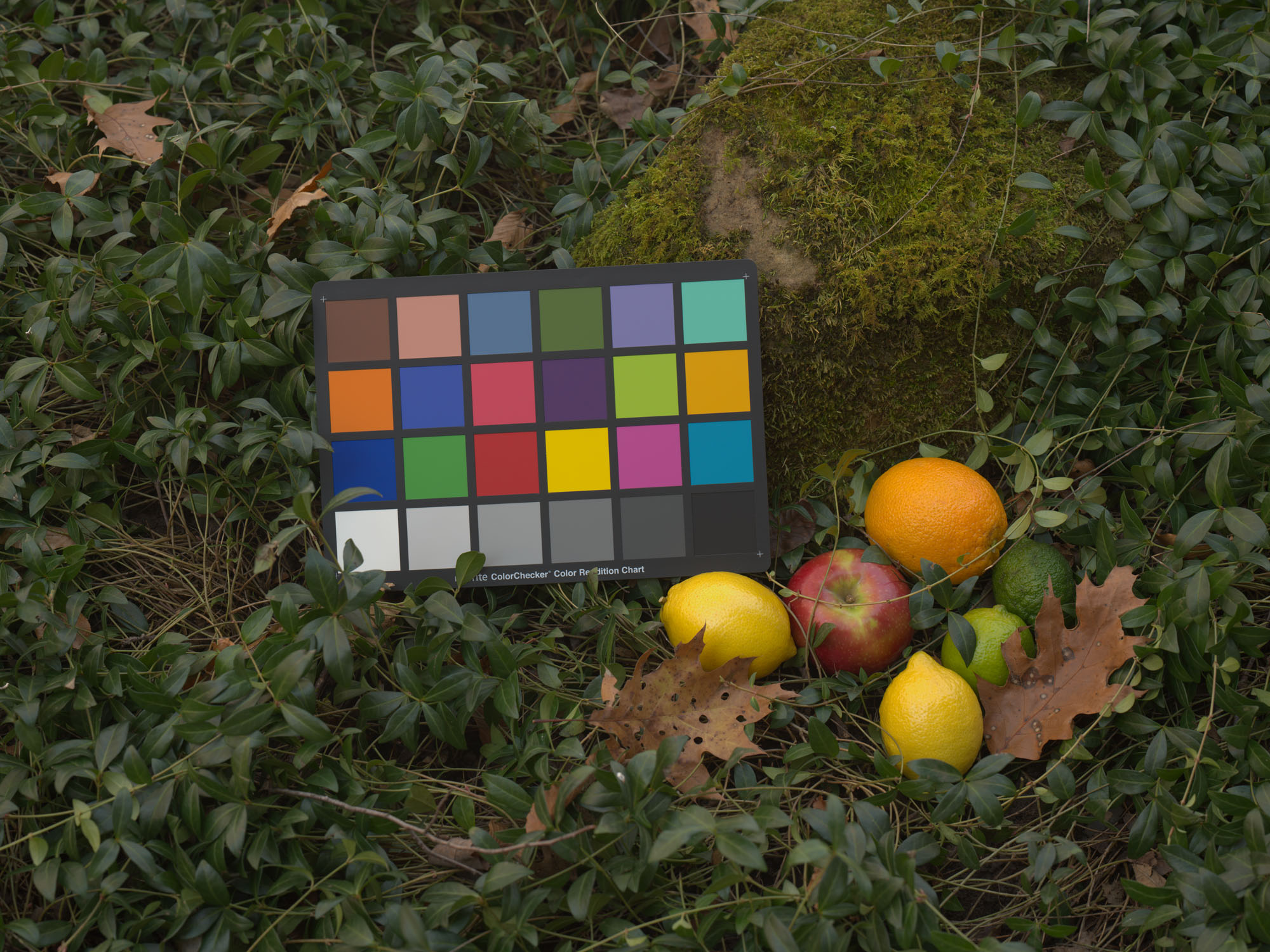
Let’s start with the compromise color matrices we derived from David Chew’s captures of a ColorChecher 24 in the shade of a sunny November morning in Ohio[2]. These are the matrices necessary to convert white balanced raw data to the perceptual CIE XYZ color space, where it is said there should be one-to-one correspondence with colors as perceived by humans, and therefore where most measurements are performed. They are optimized for each back in the current conditions but they are not perfect, the reason for the word ‘compromise’ in their name:

Continue reading Phase One IQ3 100MP Trichromatic vs Standard Back Linear Color, Part III
We have seen in the last post that Phase One apparently performed a couple of main tweaks to the Color Filter Array of its Medium Format IQ3 100MP back when it introduced the Trichromatic: it made the shapes of color filter sensitivities more symmetric by eliminating residual transmittance away from the peaks; and it boosted the peak sensitivity of the red (and possibly blue) filter. It did this with the objective of obtaining more accurate, less noisy color out of the hardware, requiring less processing and weaker purple fringing to boot.
Both changes carry the compromises discussed in the last article so the purpose of this one and the one that follows is to attempt to measure – within the limits of my tests, procedures and understanding[1] – the effect of the CFA changes from similar raw captures by the IQ3 100MP Standard Back and Trichromatic, courtesy of David Chew. We will concentrate on color accuracy, leaving purple fringing for another time.
Continue reading Phase One IQ3 100MP Trichromatic vs Standard Back Linear Color, Part II
It is always interesting when innovative companies push the envelope of the state-of-the-art of a single component in their systems because a lot can be learned from before and after comparisons. I was therefore excited when Phase One introduced a Trichromatic version of their Medium Format IQ3 100MP Digital Back last September because it could allows us to isolate the effects of tweaks to their Bayer Color Filter Array, assuming all else stays the same.

Thanks to two virtually identical captures by David Chew at getDPI, and Erik Kaffehr’s intelligent questions at DPR, in the following articles I will explore the effect on linear color of the new Trichromatic CFA (TC) vs the old one on the Standard Back (SB). In the process we will discover that – within the limits of my tests, procedures and understanding[1] – the Standard Back produces apparently more ‘accurate’ color while the Trichromatic produces better looking matrices, potentially resulting in ‘purer’ signals. Continue reading Phase One IQ3 100MP Trichromatic vs Standard Back Linear Color, Part I
What are the basic low level steps involved in raw file conversion? In this article I will discuss what happens under the hood of digital camera raw converters in order to turn raw file data into a viewable image, a process sometimes referred to as ‘rendering’. We will use the following raw capture by a Nikon D610 to show how image information is transformed at every step along the way:
