The Raspberry Pi Foundation recently released an interchangeable lens camera module based on the Sony IMX477, a 1/2.3″ back side illuminated sensor with 3040×4056 pixels of 1.55um pitch. In this somewhat technical article we will unpack the 12-bit raw still data that it produces and render it in a convenient color space.
Figure 1. 12-bit raw capture by Raspberry Pi High Quality Camera with 16 mm kit lens at f/8, 1/2 s, base ISO. The image was loaded into Matlab and rendered Half Height Nearest Neighbor in the Adobe RGB color space with a touch of local contrast and sharpening. Click on it to see it in its own tab and view it at 100% magnification. If your browser is not color managed you may not see colors properly.
We have seen that deconvolution by naive division in the frequency domain only works in ideal conditions not typically found in normal photographic settings, in part because of shot noise inherent in light from the scene. Half a century ago William Richardson (1972)[1] and Leon Lucy (1974)[2] independently came up with a better way to deconvolve blurring introduced by an imaging system in the presence of shot noise. Continue reading Elements of Richardson-Lucy Deconvolution→
Over the last two posts we’ve been exploring some of the differences introduced by tweaks to the Color Filter Array of the Phase One IQ3 100MP Trichromatic Digital Back versus its original incarnation, the Standard Back. Refer to those for the background. In this article we will delve into some of these differences quantitatively[1].
Let’s start with the compromise color matrices we derived from David Chew’s captures of a ColorChecher 24 in the shade of a sunny November morning in Ohio[2]. These are the matrices necessary to convert white balanced raw data to the perceptual CIE XYZ color space, where it is said there should be one-to-one correspondence with colors as perceived by humans, and therefore where most measurements are performed. They are optimized for each back in the current conditions but they are not perfect, the reason for the word ‘compromise’ in their name:
Figure 1. Optimized Linear Compromise Color Matrices for the Phase One IQ3 100 MP Standard and Trichromatic Backs under approximately D65 light.
We have seen in the last post that Phase One apparently performed a couple of main tweaks to the Color Filter Array of its Medium Format IQ3 100MP back when it introduced the Trichromatic: it made the shapes of color filter sensitivities more symmetric by eliminating residual transmittance away from the peaks; and it boosted the peak sensitivity of the red (and possibly blue) filter. It did this with the objective of obtaining more accurate, less noisy color out of the hardware, requiring less processing and weaker purple fringing to boot.
Both changes carry the compromises discussed in the last article so the purpose of this one and the one that follows is to attempt to measure – within the limits of my tests, procedures and understanding[1] – the effect of the CFA changes from similar raw captures by the IQ3 100MP Standard Back and Trichromatic, courtesy of David Chew. We will concentrate on color accuracy, leaving purple fringing for another time.
Figure 1. Phase One IQ3 100MP image rendered linearly via a dedicated color matrix from raw data without any additional processing whatsoever: no color corrections, no tone curve, no sharpening, no nothing. Brightness adjusted to just avoid clipping. Capture by David Chew.
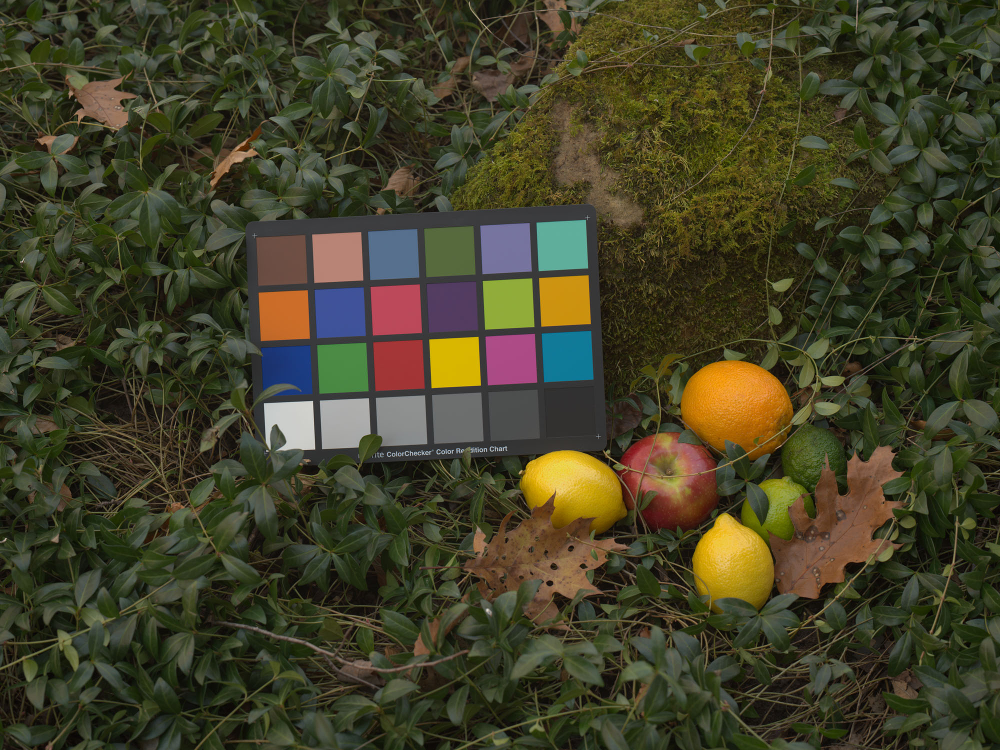
Now that we know how to create a 3×3 linear matrix to convert white balanced and demosaiced raw data into connection space – and where to obtain the 3×3 linear matrix to then convert it to a standard output color space like sRGB – we can take a closer look at the matrices and apply them to a real world capture chosen for its wide range of chromaticities.
Figure 1. Image with color converted using the forward linear matrix discussed in the article.
We understand from the previous article that rendering color with Adobe DNG raw conversion essentially means mapping raw data in the form of triplets into a standard color space via a Profile Connection Space in a two step process
The first step white balances and demosaics the raw data, which at that stage we will refer to as , followed by converting it to Profile Connection Space through linear projection by an unknown ‘Forward Matrix’ (as DNG calls it) of the form
How do we translate captured image information into a stimulus that will produce the appropriate perception of color? It’s actually not that complicated[1].
Recall from the introductory article that a photon absorbed by a cone type (, or ) in the fovea produces the same stimulus to the brain regardless of its wavelength[2]. Take the example of the eye of an observer which focuses on the retina the image of a uniform object with a spectral photon distribution of 1000 photons/nm in the 400 to 720nm wavelength range and no photons outside of it.
Because the system is linear, cones in the foveola will weigh the incoming photons by their relative sensitivity (probability) functions and add the result up to produce a stimulus proportional to the area under the curves. For instance a cone may see about 321,000 photons arrive and produce a relative stimulus of about 94,700, the weighted area under the curve:
Figure 1. Light made up of 321k photons of broad spectrum and constant Spectral Photon Distribution between 400 and 720nm is weighted by cone sensitivity to produce a relative stimulus equivalent to 94,700 photons, proportional to the area under the curve
What are the basic low level steps involved in raw file conversion? In this article I will discuss what happens under the hood of digital camera raw converters in order to turn raw file data into a viewable image, a process sometimes referred to as ‘rendering’. We will use the following raw capture by a Nikon D610 to show how image information is transformed at every step along the way:
Figure 1. Nikon D610 with AF-S 24-120mm f/4 lens at 24mm f/8 ISO100, minimally rendered from raw by Octave/Matlab following the steps outlined in the article.
In the last few posts I have made the case that Image Quality in a digital camera is entirely dependent on the light Information collected at a sensor’s photosites during Exposure. Any subsequent processing – whether analog amplification and conversion to digital in-camera and/or further processing in-computer – effectively applies a set of Information Transfer Functions to the signal that when multiplied together result in the data from which the final photograph is produced. Each step of the way can at best maintain the original Information Quality (IQ) but in most cases it will degrade it somewhat.
IQ: Only as Good as at Photosites’ Output
This point is key: in a well designed imaging system** the final image IQ is only as good as the scene information collected at the sensor’s photosites, independently of how this information is stored in the working data along the processing chain, on its way to being transformed into a pleasing photograph. As long as scene information is properly encoded by the system early on, before being written to the raw file – and information transfer is maintained in the data throughout the imaging and processing chain – final photograph IQ will be virtually the same independently of how its data’s histogram looks along the way.
I’ve mentioned in the past that I prefer to take spatial resolution measurements directly off the raw information in order to minimize often unknown subjective variables introduced by demosaicing and rendering algorithms unbeknownst to the operator, even when all relevant sliders are zeroed. In this post we discover that that is indeed the case for ACR/LR process 2010/2012 and for Capture NX-D – while DCRAW appears to be transparent and perform straight out demosaicing with no additional processing without the operator’s knowledge.


 connection space – and where to obtain the 3×3 linear matrix to then convert it to a standard output color space like sRGB – we can take a closer look at the matrices and apply them to a real world capture chosen for its wide range of chromaticities.
 triplets into a standard color space via a Profile Connection Space in a two step process
![\[ Raw Data \rightarrow XYZ_{D50} \rightarrow RGB_{standard} \]](https://i0.wp.com/www.strollswithmydog.com/wordpress/wp-content/ql-cache/quicklatex.com-164bf80016fc459bad893b6930883830_l3.png?resize=298%2C15&ssl=1 "Rendered by QuickLaTeX.com")
![\begin{equation*} \left[ \begin{array}{c} X_{D50} \\ Y_{D50} \\ Z_{D50} \end{array} \right] = \begin{bmatrix} a_{11} & a_{12} & a_{13} \\ a_{21} & a_{22} & a_{23} \\ a_{31} & a_{32} & a_{33} \end{bmatrix} \left[ \begin{array}{c} r \\ g \\ b \end{array} \right] \end{equation*}](https://i0.wp.com/www.strollswithmydog.com/wordpress/wp-content/ql-cache/quicklatex.com-f4f3535c40e6f7d83ee139eaf9633956_l3.png?resize=273%2C64&ssl=1 "Rendered by QuickLaTeX.com")
 coefficients of this matrix
  is the main subject of this article
 ,
,  or
or  ) in the fovea produces the same stimulus to the brain regardless of its wavelength
