We have seen that deconvolution by naive division in the frequency domain only works in ideal conditions not typically found in normal photographic settings, in part because of shot noise inherent in light from the scene. Half a century ago William Richardson (1972)^[1] and Leon Lucy (1974)^[2] independently came up with a better way to deconvolve blurring introduced by an imaging system in the presence of shot noise.

They asked themselves: given a noisy/blurred captured image () and a known system blurring function (), what is the most likely uncorrupted original object image ()?  That’s also what we want to accomplish because the blurring function would then have been undone, effectively performing deconvolution in the presence of noise.

The answer they came up with is robust and still being used today.  Interestingly, if it were published today it could be categorized under the artificial intelligence/machine learning umbrella. The subject is a bit dry but it’s not hard to understand and the result is surprisingly elegant.

Poissonian Light and Photoelectrons

The premise is simple and goes to the very heart of the nature of light.  We know from the dedicated article that light is emitted, arrives  at and is detected by our digital photographic sensors not in a continuous fashion but discretely, as described by Poisson statistics.  In other words for photons emitted by a stable light source arriving on the area of a pixel at a rate that would result in an average of 5.2 photoelectrons per exposure, the number of photoelectrons (e-) actually captured by such a pixel during each such exposure is not a constant 5.2 but it has a probability of achieving a given count according to the following integer distribution, aptly known as a Poisson Distribution:

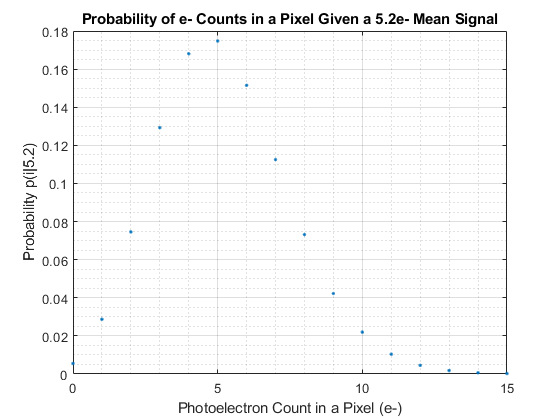
So for a given Exposure the number of photons and, more relevantly here, photoelectrons collected by each pixel in our digital sensors could literally be any integer number from zero to huge, though it’s more probable that it would be relatively close to the mean.  For instance in this example there is about a 50% chance that the number of counted e- would be 4, 5 or 6, just add up the relative probabilities.  Such deviation from a mean signal as a result of the quantum nature of photoelectrons is called shot noise in photography, the standard deviation of which is known to be the square root of the mean.

Single Pixel Stats

What is the probability that a pixel collect a given number of photoelectrons?   With exposure resulting in photoelectrons per pixel on average, the probability that a given pixel will collect photoelectrons during exposure is

(1)  

Equation (1) is the well known Poisson Probability Mass Function with

• the probability that photoelectrons will have been counted by a given pixel during exposure, and
• the mean number of photoelectrons per pixel for the given exposure.

For example with a 5.2 e- mean the probability that a pixel collect 3 e- is

   

as seen in the plot above.  Note that the mean, , is a non-negative real number (i.e. floating point) but the count, , is a discrete non-negative integer, such is the nature of quantum mechanics as it applies to light and photoelectrons.

Achieving Lambda

The problem that Richardson and Lucy tried to solve is the inverse of that exposed just above: knowing the actual measured count of a pixel (a consequence of linear light intensity on the sensing plane being recorded in the captured file)^[4], how do we find the original mean signal associated with it?  That mean would represent the ideal image not subjected to  shot noise, what they set out to achieve.

Intuitively it is obvious that if we look at a single pixel in isolation the answer could literally be anything so in that case the problem does not have a well defined solution.  But if we have more than one pixel we can start making more probable educated guesses, the more the pixels the more probably accurate the guesses.

The good thing about digital photography is that we typically have millions of pixels to throw at the problem in the form of the x array of image intensities captured (),  so millions of recorded ‘s to help us estimate associated ‘s, the ensemble of which is ideally the x image () uncorrupted by shot noise.  With just one we’d go nowhere but with millions of them we can come up with a plan, call it an algorithm.

Whole Image Stats

In what follows lower case symbols (like ) refer to individual pixels while uppercase ones refer to a whole image array of them (like ).  For the formally minded – with from 0 to -1 rows and from 0 to -1 columns – represents the intensity at every pixel in the x image,  the and indices dropped for readability (here but also for related image variables , and ).

The probability of two independent  events occurring is the product of their individual probabilities.  For instance the probability of picking a Queen of Hearts out of a deck of cards is the probability of picking a Queen multiplied by the probability that its suit is Hearts: 4/52 * 1/4 = 1/52 (of course).  This is known as a joint probability.

Using Equation (1) above we can calculate the probability that the value recorded by each pixel in the image file refers to a guesstimated mean signal associated with it.  The joint probability over the whole image is the product of the individual pixel probabilities .  Therefore is in fact an overall indication of how well the ensemble of the guesstimated x ‘s  () explains the ensemble of thex captured pixel data ‘s  ().  The joint probability for the whole image is Equation (1) expressed as a product of the probability associated with every pixel in the image:

(2)  

with

• , a scalar representing the joint probability of all individual pixels per Equation (1)
• , x captured linear image data, shot noise and all
• , x version of uncorrupted by shot noise
• , the symbol for product, meaning that the x values resulting from what follows should be multiplied together
• .  and / indicate element-wise multiplication and division respectively.

Equation (2) effectively instructs us to calculate the probability at every pixel with Equation (1) and multiply all the results together, obtaining a single joint probability value for the entire image.

Maximum Likelihood

It is obvious that if we want to maximize the probability that image data is well explained by the guesstimated uncorrupted image all we have to do is maximize .  Having achieved that, ideally the difference between images and should just be shot noise.

With a couple of tricks it turns out that maximizing is not as complex as originally suspected when Equation (2) came into the picture.  The first trick is to take the natural logarithm of both of its sides.  We can do this because the maxima of a surface and their logarithm coincide, as do their minima.  With logarithms exponents become factors and products become sums so now we need to maximize this simpler equation instead:

(3)  

Note that summation has replaced the product symbol. The job is to vary our estimated uncorrupted image () until is maximized, meaning that there is maximum chance that captured image data () is a consequence of it.  This is called Maximum Likelihood Estimation.

Bait and Switch

Since we notice that the last term in Equation (3) is a constant offset that does not vary with , it does not affect when the maximum occurs so we can drop it.  This is of course also true of any constant factors built into any of the terms, especially gain linking  captured linear image data to photoelectron counts.  It allows us to apply the described approach to image data in DN even though in that form it typically does not directly obey Poisson statistics^[4][5].

Also the negative of a maximum is a minimum so we can take the negative of Equation (3) and minimize that.  Finally, and crucially, we know that the image of the guesstimated clean signal on the sensing plane () is in fact ideally the unblurred original image of the scene without shot noise () blurred by the of the lens and imaging system

(4)  

so that

(5)  

with shot noise and two dimensional convolution.  Applying all of the above to Equation (3), and using the standard symbol for a loss function , we come up with a relatively simple final equation to minimize

(6)  

where the product and the natural logarithm are element-wise.  In classic RL deconvolution the blurring function () and captured linear image data () are known and fixed so all we need to do to estimate unblurred original scene image is to minimize by varying .  Conveniently, it turns out that the right hand side of Equation (6) is a convex function and it always has a minimum.

Minimum Unlikelihood

The process of maximizing the likelihood of the captured image data assuming a Poisson process and the given effectively yields our originally stated objective, deconvolved image – as a byproduct.

It’s obviously a calculation intensive procedure but the calculations are not difficult: take a guess at the intensities in ideal image and convolve it with the ; subtract the element-wise product of captured linear image data with the logarithm of the above and sum up such results from all pixels to obtain the unlikelihood measure .  Continue guessing variations on systematically until the unlikelihood is minimized, et voilà RL deconvolution achieved while keeping shot noise under control.

So how do we do the systematic guessing efficiently?  Hmm, where have I seen cost functions similar to Equation (6) before?  Next.

 

Notes and References

<sub>1. Bayesian-Based Iterative Method of Image Restoration, William Hadley Richardson, Optical Society of America (1972).
2. An iterative technique for the rectification of observed distributions, Lucy, L. B., Astronomical Journal, Vol. 79, p. 745 (1974)
3. This paper by Dey et al. (2004) has a good review of the theory underlying this and other similar algorithms.
4. For simplicity assume a monochrome sensor in this post.  Linear image data captured in the file in DN is related to photoelectron count by a factor, gain. This means that the data needs to be divided by gain (DN/e-) in order to obey Poisson statistics directly.  Actual re-scaling of image data  to e- is however superfluous as a consequence of the logarithm in Equation (3), which effectively turns gain into a constant offset that does not alter the location of the maximum/minimum.
5. With logarithms exponents become factors so we should be able to use gamma encoded data as-is, producing a gamma encoded result, because the gamma exponent will simply multiply every DN by a constant and the maximum will still occur when is the most likely explanation for a gamma encoded .  However, it would not work properly with gamma functions with a linear toe, like sRGB.
6. The process described does not minimize random read noise in the deep shadows (nor PRNU) though it should be noted that a Poisson distribution approaches a Gaussian distribution starting from fairly low levels of light in typical photographic applications.
7.  The exact same thought process that was used here assuming Poisson noise can be used to derive a different cost function that assumes Gaussian noise throughout instead, as explained by Dey et al, in the reference above.</sub>