We understand from the previous article that rendering color with Adobe DNG raw conversion essentially means mapping raw data in the form of  triplets into a standard color space via a Profile Connection Space in a two step process
![\[ Raw Data \rightarrow XYZ_{D50} \rightarrow RGB_{standard} \]](https://i0.wp.com/www.strollswithmydog.com/wordpress/wp-content/ql-cache/quicklatex.com-164bf80016fc459bad893b6930883830_l3.png?resize=298%2C15&ssl=1 "Rendered by QuickLaTeX.com")
The first step white balances and demosaics the raw data, which at that stage we will refer to as , followed by converting it to  Profile Connection Space through linear projection by an unknown ‘Forward Matrix’ (as DNG calls it) of the form
(1) ![\begin{equation*} \left[ \begin{array}{c} X_{D50} \\ Y_{D50} \\ Z_{D50} \end{array} \right] = \begin{bmatrix} a_{11} & a_{12} & a_{13} \\ a_{21} & a_{22} & a_{23} \\ a_{31} & a_{32} & a_{33} \end{bmatrix} \left[ \begin{array}{c} r \\ g \\ b \end{array} \right] \end{equation*}](https://i0.wp.com/www.strollswithmydog.com/wordpress/wp-content/ql-cache/quicklatex.com-f4f3535c40e6f7d83ee139eaf9633956_l3.png?resize=273%2C64&ssl=1 "Rendered by QuickLaTeX.com")
with data as column-vectors in a 3xN array. Determining the nine  coefficients of this matrix
  is the main subject of this article[1].
The second step projects the resulting image information from to the ‘output’ colorimetric color space chosen by the photographer, say sRGB or Adobe RGB. The necessary linear matrices for this transformation are standardized and readily available online.
9 Equations and 9 Unknowns
So how do we determine the nine coefficients of the Forward Matrix in Equation 1?
The 9 unknown coefficients operate on white balanced and demosaiced data to transform it linearly into data. It follows that if we had three sets of values under  illumination and we knew their corresponding triplets we could solve for the coefficients. The results would be valid for the given hardware, scene and lighting.
For instance we could capture in the raw data 3 patches of uniform diffuse reflectance illuminated by a light source with the camera whose matrix we want to determine, thus obtaining three sets of values; then measure with a spectrophotometer or similar instrument the reflectance of the 3 patches and illuminant spectral power distribution; and calculate the values that the reflectance and illuminant imply.
All that would be left to do then is assemble the 3×3 pairs of and corresponding data per Equation (1) and multiply it out. Below the ‘s that make up are the unknowns, the X,Y,Z’s and  ‘s would be known:
(2) 
9 equations and 9 unknowns provide a guaranteed solution for the coefficients of the relative Forward Matrix . Looks easy? In fact it is much easier than that.
1 Capture, 72 Equations
X-Rite produces a number of ColorChecker 24 patch standard targets whose reflectance information is published and well thumbed. For this example I will use their handy Passport Photo version.
The 24 patches in the ColorChecker target carry reflectances that are supposed to be representative of everyday photographic subjects, as found in skin, foliage and sky colors. The color scientists at BabelColor.com have measured a sample of 30 ColorChecker targets over the years and compared them to published specifications (pre-November 2014 formulations shown, as my unit is older than that)[2]:

Note that 1  is supposed to represent a just noticeable color difference, so you can see that with the exception of purple and white the patches do seem to provide a reasonably stable reference. This information, as well as average patch reflectance from 380 to 730nm at 10nm increments, is available in a spreadsheet from the relative link above.
Bingo! the L*a*b* color space is a simple transformation away from . With the data above and a single raw capture of a ColorChecker Passport Photo target in clear noonish sunlight (call it D50) we’ve got 24 as opposed to just 3 sets of raw and reference data triplets needed to solve for the coefficients of the Forward Matrix in Equation 1, making the system overdetermined. We can use the larger data set to make sure that the coefficients fit a wider number of potential photographic subjects – that’s why they call it a compromise color matrix. Shutter Release.

Computing the Coefficients by the Normal Equation
Ok, so now we have the cc24 target illuminated by a roughly D50 source captured in the raw file of a Nikon D610+24-120mm/4. Next we read the mean  values in the three color channels for each of the 24 patches with a tool like RawDigger [3]. Then we white balance them based on the third gray patch from the right in the neutral bottom row and demosaic them. The result is now the white balanced and demosaiced raw data set that we need, one triplet per patch.
We could then obtain the reference corresponding to each patch by measuring them or via ColorChecker values published by X-Rite or BabelColor as above and solve the 72 equations for the coefficients in matrix that best fit the available data using the Normal Equation. To be consistent with the format of matrix multiplication and Equation (1) the solution can be shown as follows:
(3) ![\begin{equation*} M = [inv(rgb^T * rgb)*rgb^T*XYZ_{D50}]^T \end{equation*}](https://i0.wp.com/www.strollswithmydog.com/wordpress/wp-content/ql-cache/quicklatex.com-57425decd30e32eea69fd5589326cacb_l3.png?resize=319%2C22&ssl=1 "Rendered by QuickLaTeX.com")
with  representing the transpose,
  the inverse of the relative arrays and data Nx3, as you will find it in the Matlab script linked in the notes. Voilà, by the magic of linear algebra Equation 3 will produce the 3×3 compromise color matrix resulting in the smallest sum of square differences to reference values for the target as measured (if you would like more detail on this subject you may be interested in the article on Color Transforms).
However that turns out not to be the best way to solve for because the method gives equal weight to all tones, while the Human Visual System tends to be more sensitive in some parts of the XYZ color space than others.
A Better Color Difference Metric: dE2000
In fact in what follows I will use the standard color difference (CIEDE2000) as the minimization criterion. We can set up a spreadsheet with the 24 triplets and 9 cells representing the coefficients in the forward matrix as arrays. Seed the coefficients with the result from Equation (3) above to get us in the ballpark. Matrix multiply the triplets by the seed matrix, convert to L*a*b*, compute differences to the reference values in Figure 1 above and let Excel Solver figure out what values of the 9 coefficients of minimize the sum of the differences. The resulting matrix will be the best compromise found for the 24 patches under that illuminant, taking HVS color sensitivity in consideration therefore giving each patch approximately equal perceptual importance.
The Compromise Forward Matrix
I effectively followed that last procedure but using Matlab/Octave instead of Excel, if you would like to follow along you can download the routine I used from the relative note at the bottom of the article. Excellent toolkit OptProp and its built-in ColorChecker reference data lent a helping hand[4]. This is the Forward Matrix obtained for my setup:
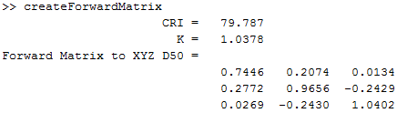
Cool. These are the differences for each patch resulting from the transformation using OptProp’s ColorChecher reference data.

The average is 1.5 and maximum is 3.8 in the light skin patch. Recall that 1 is a just noticeable difference. I repeated the exercise this time using the BabelColor 30 database as reference and this is the resulting forward matrix then:
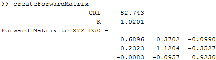
Looks like the differences to reference data from BabelColor’s database are more evenly distributed: average is still 1.5 but Maximum is a lower 3.1 in the ‘green’ patch.

To do it properly I should have measured the Spectral Power Distribution of the illuminant and the reflectance of the patches with a spectrophotometer around the time that the capture was taken (didn’t have one, X-Rite ColorMunki Photo on the way, see post scriptum). Using published reference SPDs and reflectances pollute the data and contribute to degrade the results – but you get the idea.
Correcting Matrix ‘Errors’: Profiles
Note however that the compromise matrix is just that, a compromise, and even if the procedure had been perfect it could result in relatively large errors. For better overall color rendering performance the preferred method is to correct such errors through optional nonlinear color profile adjustments that are typically introduced while in via ProPhoto RGB HSV lookup tables. The tables and application methods are usually referred to as camera ‘profiles’ (ICC and DCP for instance), a subject beyond the scope of this article[5].
Calculating Sensitivity Metamerism Index (SMI)
While the data is out we can calculate the Sensitivity Metamerism Index, which for us is equal to 100 minus 5.5 times the average  (not ) of just the 18 color patches[6]. The shown values (misnamed CRI above) are not necessarily maximized for the given setup because the matrix finding routine is built upon minimizing . Still my D610 with its 24-120mm/4 around D50 shows SMIs of 80 in the first case and 83 in the second. They jump to 82 and 86 respectively if the routine is setup to minimize instead. Not bad, although I know some people do not give much credence to single figure metrics – and I can see why.
Step 2: Matrix to Output Color Space
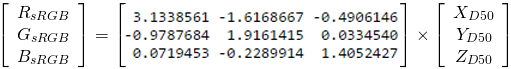
Now that we have done the hard work of determining the Forward Matrix to convert white balanced raw data to the PCS with this illuminant, we need a standard matrix to move it on to the colorimetric color space chosen by the photographer for output. In this case we will map it to  by multiplication with the following transform matrix obtained from Bruce Lindbloom’s site[7]
The product of this and the forward matrices calculated earlier produces the following combined white balanced raw  linear transforms for a D50ish illuminant. My results are shown top and bottom, with DXOmark’s for the D610 at D50 in the center for reference[8]:

Pretty close, which confirms the illuminant of my captures was indeed near D50.
So that’s where color matrices come from and why we need them. Next, a closer look and putting them to work.
Post Scriptum
I got myself an X-Rite ColorMunki Photo spectrophotometer [Edit: its hardware is supposed to be identical to the rebranded i1 Studio aka Calibrite ColorChecker Studio], it’s a blast. It comes with a ColorChecker Classic Mini, I assume with the new formulation. I measured it with the Munki using open source spotread from ArgyllCMS and captured it in the raw data in somewhat similar conditions to Figure 2. Correlated Color Temperature was about 5050K. These are the matrices that are produced from it (white balanced off my WhiBal card):
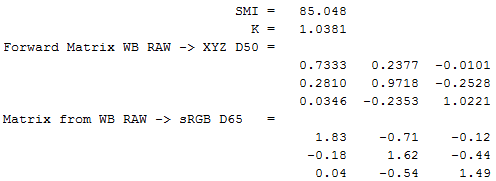
Pretty similar and SMI is now 85. In fact if I set the routine up to minimize instead of SMI is 86. The sum of rows in the XYZ matrix should represent the white point of the target illuminant, which in this case was just the reference data for D50. The matrix white point is [0.9609 1 0.8214] which has a correlated color temperature of 5016K, according to Bruce. Good, because D50 has a CCT of 5002K.
Here are the differences, measured vs captured:

Now average is 1.17, there are only three patches above 2 and the rest seem to be better controlled overall. I guess pushing down the outliers is the reason why linear matrices are not enough and profiles are necessary. To get even closer I should have brought the Munki with me and measured the illuminant. Well, next time.
Notes and References
1. Lots of provisos and simplifications for clarity as always. I am not a color scientist, so if you spot any mistakes please let me know.
2. The ColorChecker pages at BabelColor.com can be found here. Careful that there was a change in formulations in November 2014.
3. RawDigger can be found here and dcraw here.
4. optprop can be found here.
5. For an example of profile implementation see for instance Adobe’s Digital Negative Specification Version 1.4.0.0.
6. See here for a description of the Sensitivity Metamerism Index and here for DXO’s take on it.
7. See this page at Bruce Lindbloom’s site for precise matrices from XYZD50 to many colorimetric color spaces.
8. DXOmark.com D610 color measurement can be found here by clicking on the ‘color response’ tab.
9. The Matlab/Octave matrix finding routine I used can be downloaded from here., there is some discussion of the code in this thread. If you have any questions let me know in the comments or via the form in the About page, top right.
Is there any relevant source code that can send a copy to my mailbox? thank you very much
Sure, I emailed the Forward Matrix to XYZn code to you. Any questions let me know.
Good work
Currently we use x-rite 24 patch, using least squares fit *L.
Then use grey 6 for luminance balance, 6 primaries (row up from greys) for hue/sat correction.
Curious have you tried weighting patches based on Luminance, suspect if below a luminance it should be ignored.
Having to work out colour matrix due to processing raw photos.
Hello Brad,
The loss function that is minimized above is de2000, which is based on all three variables (L*, a and b) so it does take L* into consideration as-is. It shouldn’t make any difference to the end result if one is consistent throughout but before feeding linear data to the minimization routine, XYZ data is normalized so that the patch 22 Y channel measured vs reference are the same. Patch 22 should be about neutral and around 20% reflectance, so close to mid-gray.
Hi, Could you send me a copy that source code? It would be very helpful to understand it more. Thank you very much
Hi Hilly, sent.
Hi Jack,
I highly appreciate all of your posts, very educational to me.
I am having some difficulties translating the math, could you please send me a copy of the source code? It help a lot.
Thank you.
Essam
Hi Essam, sent. I have also added a link to it in the text and the notes above since I keep getting requests for it.
This is the most comprehensive and awesome set of posts I have seen on a range of technical subjects. I have only scratched the surface, having gotten to this site looking for informative description of digital camera raw processing.
Thank you for sharing your knowledge in this way.
My pleasure, thank you Allen (:blush:)
Jack it sounds like you worked through this in excel …would you be willing to share that sheet…..I sort of follow things but having a worked example in a ss to confirm that I understand would be a benefit.
Thanks
Hi Todd, unfortunately I soon switched to Matlab and the original Excel sheet is nowhere to be found. If you read Matlab you can see the routine I use in the Notes just above Comments.
Hello Jack,
If I have filters spectrum how can I reconstruct the image colors from them? How the matrices will look like?
Hi Mansoor,
It works the same as described in the article, except that the raw data is generated artificially by elementwise multiplication of the following spectral data: illuminant(s) * patch reflectance(s) * CFA. Then calculate reference XYZ values for each patch to be used in the fit by replacing CMFs for the CFA in the spectral calculation above and proceed to calculate the appropriate matrix.
Ideally two matrices should be obtained for two illuminants representing the extremes of the typical working range (the DNG spec uses A and D65), based on a wide range of patches for which reflectances are known. One set of known reflectances are those found in the BabelColor’s CC24 spreadsheet linked in the References. But the larger the set the better.
Jack
Absolutely excellent, Jack!
Why thank you Ted, nice of you to drop in.
Hi Jack,
Thank you for an excellent walk-through of steps for determining a forward matrix.
I have downloaded your MATLAB code and have a couple of questions that I hope you can shed some light on:
1) In a previous answer to a question asked back in July 2019, you touch upon the normalization that you perform on line 17 in your code:
raw = raw ./ raw(22,:) * xyzRef(22,2); %normalize wbraw
Can you explain why you do that? Is is necessary for the minimization to converge?
2) On line 22 in your code, where you specify the minimization function, you multiply “raw” with the transpose of M (M’). Why do you do that, as not multiplying with the transpose of M, would just provide you with the transposed matrix in the output. Maybe we are down to conventions of how to represent a forward matrix? Which would mean that the forward matrix should ALWAYS be transposed before being multiplied with a RGB value?
3) My final question relates to the normalization of M on lines 25 and 26. Why do you make that final normalization the resulting forward matrix?
An then just a small comment: In equation 3, you are missing a transpose on the third occurrence of “rgb” 😊. Line 21 in your MATLAB code showing the transpose (which is required for the equation to compute).
Thanks,
Henrik
Hi Henrik,
You are absolutely correct about the missing transpose in Equation 3, typo corrected, thanks! As for your questions:
1) Line 17 white balances the data and normalizes it so that it has the same intensity as Y in the reference target patch. I have chosen patch 22 because it is around mid-gray but you could use other neutral ones. It’s not necessary for covergence, but if you do not white balance the raw data before running the fit the resulting matrix is no longer going to be wbraw->xyz (Mf) as required by the DNG spec but unbalanced raw->xyz (Mu) instead. The two are related by white balance multipliers (mult) as follows: Mu = Mf * diag(mult)
2) The matrix multiplication convention used throughout the article is shown in Equation (1). Since the raw data is expected to be Nx3 by the routine, it needs to be transposed so the operation is M * raw’. This is the same as raw * M’. The second formulation is preferable when there is a lot of data to multiply because it only needs to transpose the 9 elements of the matrix. Not necessarily a worry here but imagine doing matrix multiplication over a whole image.
3) The normalization in lines 25 and 26 ensures that the sum of the Y row of the matrix adds to one. That’s necessary so that the overall brightness of the image is not changed with multiplication by the forward matrix because as you know Y is ideally proportional to Luminance in cd/m^2. I extract the factor k in line 25 just to measure how close the optimized/compromised result got to the normalization in your first question. It should be within a few percentage points or it’s possibly an indication that something is not right.
Hope it helps,
Jack
Hi Jack,
Excellent! Thank you for your thorough replies which all make good sense!
Kind regards,
Henrik
Hi Jack,
I stumbled into this googling something that I’d read on a forum (that the adobe .dcp files have forwarding matrixes, but the embedded profile in the dng of the camera doesn’t)
Forum chap said he could calculate the forwarding matrix (presumably) based on the info in the colour matrix…
Anyway I can’t begin to figure it out, although your article has at least made more sense than than adobe’s dng standards paper on the subject!
I guess failing maths back in high school DID eventually trip me up after all! 😉
Thanks again
Adam
Hello Adam,
The profile embedded in the DNG does indeed have Forward Matrices but recently they are desaturated and not useful on their own without the associated LUTs. They do this to bring as much of the ‘raw’ data into XYZ and then stretch things back out while striving to keep it in-gamut with the LUTs.
And you can indeed calculate Forward Matrices from Color Matrices, if one wants a generic matrix-only solution that may be the easiest way to go these days of desaturated FMs.
All you need to do is invert the appropriate CM (pinv in Matlab) and correct it based on the Correlated Color Temperature of the illuminant, no need to white balance the raw data first. With CCT in hand the appropriate CM is found by mired interpolation, multiplication by the relative Bradford Chromatic Adaptation matrix does the rest. Not for the faint of heart, send me a mail via the ‘About’ tab top right if you want to pursue this further.
Jack
Hello Jack,
I did contact you via the ‘About’ tab.. I suspect I was too rambling and incoherent! My apologies
I would like to give this a try.. as you’ve no doubt realised I’m struggling to get my head around the maths I need to perform, the waters are no doubt further muddied by my lack of understanding of terms such as CCT and mired interpolation..
Adobe’s DNG spec document makes this all sound moderately easy…
But articles such as yours suggest that there’s much more to it.
I’ve been using the adobe standard DCP to validate my results, in that it has a forwarding matrix, so if I can run the data from the same DCP’s colour matrix and get to the values of the forward matrix then I should be able to do the same with the embedded profile that contains no forwarding matrixes…
….but alas I can’t get close!
So here’s the data from the standard profile that has FMs
[ 0.794300, -0.259700, -0.071600 ],
[ -0.463900, 1.435700, 0.014100 ],
[ -0.058700, 0.218800, 0.760800 ]
According to the online calculator I used.. This is it inversed
[ 1.08919548, 0.18191368, 0.09913435 ],
[ 0.35210745, 0.60010052, 0.02201561 ],
[ -0.01722573, -0.15854845, 1.01990168 ]
So what do I do now?
If you can help me take my first baby steps with all of this I would be very grateful
Regards
Adam
Hi Adam,
It would take too long to explain how to reconcile FMs and CMs. If I understand correctly you are trying to generate a single matrix to take you from raw data to the final color space starting from CMs only, e.g. color matrices from dcraw. The procedure and math is relatively simple – but simplicity is relative to where one starts from 😉
1) Get a single CM valid for the correlated color temperature (CCT) of the illuminant at the time of capture.
In Digital Camera Profiles (DCP) there are normally two CMs optimized for either end of the illuminant spectrum: one matrix typically optimized for illuminant A (i.e. a light bulb, CCT=2885K) and one for D65 (i.e. shade or indoors, 6502k). From these, the one CM that will be used needs to be determined by linear interpolation, given the Correlated Color Temperature of the illuminant of the capture at hand. The interpolation occurs in mired units (i.e. 1/CCT). You can determine the CCT of the illuminant in your capture from white balance multipliers and CMs iteratively as explained by Lindbloom.
2) That gives you the matrix from XYZ at the given CCT to Camera Neutral (i.e. the raw data you would see in a neutral uniform patch, before white balancing – this is a key difference from FMs). Take the inverse of that to get the matrix we are after, from Camera Neutral to XYZcct.
3) Adapt the matrix in 2) to the viewing environment.
The matrix at this stage is ‘valid’ for the raw capture’s CCT and it needs to be adapted to the viewing conditions, typically indoors with a D65 white point. The suggested adaptation from capture CCT to 6502K is Bradford, as described by Lindbloom.
4) Now you have a matrix that takes your raw data as-is (i.e. not white balanced in contrast to FMs) to XYZ D65 so you need to convert it to the viewing color space, say sRGB, per the relative matrix found in Lindbloom.
Et voilà, the result can be packaged in a single matrix that takes demosaiced, non white balanced, raw data in your capture to the final color space.
Jack
PS The DNG spec takes a detour via D50 in 3), compensated for by an adapted matrix in 4), as described in this article. Results are the same.
Jack, very clear and helpful exposition. I was having a similar struggle trying to reconcile the Forward Matrix with the Color Matrix, and your comments about the FMs being specified in a desaturated fashion were the only explanation that I found online on the reason for the discrepancy. I am still curious on the details on how to reconcile them. Since you said it would take long to explain that, could you point me to any document or paper that provides the details? Thanks very much! -Julio
Hi Julio, I am afraid that I do not know of any document that explains it because every profile maker tends to do their own thing. Keep in mind that FMs are usually preferable to CMs for a number of reasons, so if you have one of those you are better off to go with it. If you only have CMs you can calculate a workable FM as described in the DNG spec. Just don’t expect it to be exactly the same as a FM from someone else’s profile.
Hope this helps,
Jack
Thank you Jack. So to check my understanding – if I use the FM given in the DNG file, then I need to use the tone curve (LUT) provided in the file, but if I calculate a workable FM from the CM, then I can use the standard 2.2 gamma tone curve, correct? In my experiments, I get a very low saturation image if I use the FM given in the DNG file and the standard 2.2 gamma, but if I derive the FM from the CM, and then 2.2 gamma, then the image comes out with the correct saturation. In fact, by using the FM derived from the CM I can obtain, very nearly, the matrix given in the DxO Mark website, but if I use the FM specified in the DNG file, the resulting matrix differs quite a bit from the DxO Mark one.
Correct Julio. Current Adobe generated FMs are desaturated to start with because they assume that saturation will be re-injected by the LUT after having made the jump into XYZ. This way they minimize gamut clipping there and can better manage gamut compression – albeit at the expense of linearity.
This is a great summary, but your main assumption that “clear noonish sunlight” is representative of a D50 light source is incorrect, in fact it’s closer to D65.
This link shows the spectrum of sunlight at about 9am on a clear day in Canada which closely resembles the D50 spectrum. If you don’t use the right light source, your colour matrix will be wrong.
https://whattheythink.com/articles/101096-question-daylight-really-d50-answer-yes/
You bring up a good point, Andrew.
In those days I did not have a spectrophotometer to measure the SPD of the illuminant at the scene and naively trusted CCT estimates off gray cards by raw converters like ACR and RawTherapee, which by the way is how they determine their color transforms internally. I quickly learned that these can be quite inaccurate.
I would guess that CCT in the article was somewhat higher than that suggested by D50, though given the mountain setting most likely closer to it than to D65, which is instead assumed to occur indoors and in the shade. Should anyone be interested in the errors that an incorrect guess at the CCT of the illuminant can make in daylight, see Figure 2 in this article:
https://www.strollswithmydog.com/white-balance-is-off/
Deviating from DNG conventions, a better way to estimate the color transform is to carry a gray card and a color meter and follow the process outlined in the series of articles around here:
https://www.strollswithmydog.com/white-point-cct-tint/
Jack
Thanks Jack, very helpful. I’m trying to colour balance my astrophotography camera which captures in linear space, has no auto-WB feature (just a couple of multipliers for red and blue) and it’s pretty hard to get a colour chart or grey card out into space to image during the night. I’m working on imaging a Macbeth chart under D65 or D50, then calculate a colour correction matrix in Argyll and apply that to my images of the planets (which are illuminated by the sun, but we only capture the direct sunlight, not the diffuse (blue) skylight).
Fun times 🙂
Hi there, I’m wondering if you can help me. I’m (still) trying to calibrate my astronomical camera without any success, I think I’m just missing a key piece of information here.
The images from astronomical cameras (like my ZWO ASI224MC) generate data that is uncalibrated, uncorrected and in simple linear format. I’ve used it to capture a 24 panel Gretag Macbeth colour chart in a lightbooth under D65 conditions, but I am at a loss as to how to continue. If I were to send this to you would you be able to assist me along the path?
Thanks, Andrew.
Hello Andrew,
Is that D65 a calibrated source? If not it would probably be better to take a picture of the CC24 under noonish sunlight (D55) and use that.
Once you have the 24×3 bias subtracted raw rgb samples, just use Argyll or the matlab routine in the link with the 24×3 Babelcolor reference values to compute the rgb->XYZ matrix. You can also do it in Excel, the math can be simple and it is outlined here:
https://www.strollswithmydog.com/linear-color-transforms/
If you are still having trouble let me know and I’ll give you a hand.
Jack
Thanks Jack, I don’t have Matlab and I’ve done a bunch of stuff in CoCa (Argyll) and Excel already to produce icm files and colour correction matricies with some success, but applying these in anger to my actual astro images is proving difficult. The image of the colour chart was taken using a x-rite “SpectraLight QC” light box in D65 mode, so should be fairly accurate.
I’m running this enquiry on a number of fronts (see here to where I am with another user on an astronomy website, which includes a link to my journey).
I can share the raw data image with you, any help you can provide would be very much appreciated.
Thanks again, Andrew
Hello Jack,
I have a question on the CCM: in your experiments did you notice a significant difference between the CCMs for two illuminants that have the same CCT? For instance on a LED and a Fluorescent?
I’m wondering if it makes sense to do it, or just interpolation based on CCT (with two points like in DCP or even more) is enough.
Hi Clement, apologies for the late reply, it’s the rush before Xmas.
Yes, sometimes the differences are quite large. Think of spectra as being at least 30-dimensional (400 to 700nm every 10 nm), and CCT as being two dimensional (CCT and Duv). Much can happen in 30 dimensions that does not show any change in 2. Cones in the eyes work in 3. Another name for this is metamerism.
It is better to interpolate between like sources (e.g. D illuminants, or BB radiators, but not between them).
Jack
This is terrific. I’m trying to create a DNG files for a ZWO ASI676MC Color Astronomy Camera (Sony IMX676 sensor). As far as I can tell no one has previously done that so I’m planning to follow your process. Two questions:
– would it be possible to get code the implements this?
– is there some good example code that writes a DNG file with the minimal set of tags required to have the Adobe tools process it.
Thanks so much!
Hi Matt,
you can find Matlab sample code in the notes at the bottom of this article or, better, at the bottom of this one
https://www.strollswithmydog.com/linear-color-transforms/
As for writing to DNG you should try the Adobe DNG SDK. Perhaps it’s easier to simply write the .dcb profile file, though this is not my area of expertise.
Jack