Color: From Object to Eye

How do we translate captured image information into a stimulus that will produce the appropriate perception of color? It’s actually not that complicated^[1].

Recall from the introductory article that a photon absorbed by a cone type ( $\rho$ , $\gamma$ or $\beta$ ) in the fovea produces the same stimulus to the brain regardless of its wavelength^[2]. Take the example of the eye of an observer which focuses on the retina the image of a uniform object with a spectral photon distribution of 1000 photons/nm in the 400 to 720nm wavelength range and no photons outside of it.

Because the system is linear, cones in the foveola will weigh the incoming photons by their relative sensitivity (probability) functions and add the result up to produce a stimulus proportional to the area under the curves. For instance a $\gamma$ cone may see about 321,000 photons arrive and produce a relative stimulus of about 94,700, the weighted area under the curve:

equal-photons-per-wl — Figure 1. Light made up of 321k photons of broad spectrum and constant Spectral Photon Distribution between 400 and 720nm is weighted by cone sensitivity to produce a relative stimulus equivalent to 94,700 photons, proportional to the area under the curve

To provide such a stimulus to the eye an output medium would have to either produce a similar Spectral Photon Distribution or – because the system is linear and an absorbed photon is an absorbed photon independently of wavelength – simply any other combination of photons that when integrated by a $\gamma$ cone will yield the same 94,700 photon stimulus.

So alternatively a monitor could send a signal of 94,700 photons at the peak-response wavelength of 544nm to the foveola: the eye would be none the wiser and perceive the signals of Figure 1 and 2 as identical.

photons-at-544 — Figure 2. The same cone stimulus as in Figure 1 provided by 94,700 equivalent photons at the single wavelength of 544nm.

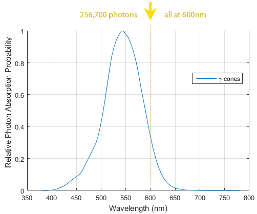
Or the monitor could send all photons at 600nm. Of course then it would have to send more photons than in the previous case because in $\gamma$ cones the probability that a photon will be absorbed is only 36.88% at that wavelength than at 544nm, so it would have to send about 256,700 photons at 600nm to obtain the desired effective stimulus of 97,400:

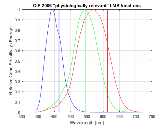
As far as the eye is concerned, the three signals are identical and, with some limitations, will produce the same stimulus to the brain. So a monitor designer could just choose one wavelength to stimulate the effect of all others on the relative cone and adjust the strength of the signal performing the simple calculation that we did above to the same effect. Such a wavelength is referred to as ‘primary’ and the underlying theory as Young-Helmholtz.

Output Trichromacy

It’s clear from this discussion that the job of an output device like a monitor has just been made much easier: to provide a perceptually ‘accurate’ response it does not need to be able to reproduce all visual frequencies in nature but just three primary ones, one per cone type. This fact was well known a hundred years ago and has been exploited to good effect ever since to produce additive color systems like color TVs. For instance, the three primaries chosen for the HDTV (and sRGB) standard correspond to about 612.5nm, 546.8nm and 464.6nm for the red, green and blue channels, respectively aimed primarily at $\rho$ , $\gamma$ and $\beta$ cones^[3].

srgb-primaries — Figure 4, HDTV is based on sRGB’s primaries, which provide trichromatic stimuli of dominant wavelengths 612.5, 546.8 and 464.6nm for the R, G and B channels respectively.

Reproducing an appropriate color then simply means being able to best translate the subset of full spectrum visual information captured by an input device into the correct strength of each of the primaries of an output device in order to reproduce in the cones the sensation of viewing the live object: for the example of the previous article when viewing green foliage, 238, 197 and 38 photons absorbed by the $\rho\gamma\beta$ cones respectively.

spd-to-cone-quanta3 — Figure 5. When observing the scene, light reaches the eye and is integrated by the three cone types to provide a tristimulus response processed by the human brain as color.

Within adapted conditions what matters most for the perception of color is the relative spectral distribution of the arriving photons – hence the ratio of the three figures – rather than their absolute numbers: for the same distribution at the eye, twice/half the number of photons will produce roughly the same perceived ‘foliage’ green.

Input Trichromacy

Not coincidentally digital cameras work fairly similarly to the eye in how they acquire color information: the Color Filter Array is composed of three filters (call them $r$ , $g$ and $b$ ) with spectral sensitivity functions that attempt to mirror the sensitivity of the three cone types. The averaged Spectral Sensitivity Functions of the CFAs of about 20 digital cameras measured by Jun Jiang et al. at the Rochester Institute of Technology^[4] are shown below left. Below right they are shown with cone responses superimposed^[5], arbitrarily scaled for ease of comparison so that all curves peak at one.

cfa-cone-ssf-comparison — Figure 6. Left 6a: Digital Camera CFA Spectral Sensitivity Functions, average of Jun Jiang et al. database, Right 6b: SSFs from the left, normalized to 1 at peak and CIE 2006 Physiologically Relevant LMS Functions.

As photons of a given spectral distribution arrive from the scene they are weighted by the sensor/CFA SSFs and integrated by each pixel, much like cones weigh them and integrate them for absorption. If the sensitivity curves of the sensor and cones were the same we would pretty well be done. But that’s not the case so the raw counts from the camera need to be adjusted accordingly. For example $rgb$ pixels exposed to the spectral distribution of ‘foliage’ green in ‘daylight’ might produce raw counts to the relative tune of 160, 197, 25 when cones in the eye of an observer at the time of capture would have instead absorbed photons producing stimulus 238, 197, 38.

Why Color Transforms Are Needed

Mapping color information from the input to the output device is what we call color transformation or conversion in photography. We refer to the set of all possible triplet combinations in the same state as a ‘space’ and the function that maps them from one space to another as a transform. We assume that the system is linear and wish to keep it that way as much as we can.

One intuitive way to deal with the transformation would be to use a lookup table: ‘a count of 160,197,25 in the raw data corresponds to cone responses of 238,197,38’. That way if the camera is exposed to green foliage in dayight it will record it in its own units in the form of a raw $rgb$ triplet, which will then be translated by the table to the correct cone stimulus for ‘foliage’ green in daylight, ready to be projected on the average observer’s eye. A specific table would of course need to be created for every illuminant and display.

Linear Algebra to the Rescue

In fact there are too many possible triplet combinations for a practical lookup table implementation and even then we would most likely loose linearity. However, Young-Helmholtz theory assumes color vision to work as a three dimensional linear system^[6] so there is an easier way: come up with an illuminant dependent linear matrix that will transform values from camera space to cone space, taking the (demosaiced) $rgb$ raw count as the input and providing the appropriate $\rho\gamma\beta$ figures to the output device – which will be assumed to be smart enough to shoot out the ‘correct’ number of photons according to its primaries in order to ‘accurately’ stimulate human cones for the color at hand:

(1) $\begin{equation*} \left[ \begin{array}{c} \rho \\ \gamma \\ \beta \end{array} \right] = \begin{bmatrix} a_{11} & a_{12} & a_{13} \\ a_{21} & a_{22} & a_{23} \\ a_{31} & a_{32} & a_{33} \end{bmatrix} \times \left[ \begin{array}{c} r \\ g \\ b \end{array} \right] \end{equation*}$

If we can figure out the nine constants ( $a$ ) that make up the $rgb$ to $\rho\gamma\beta$ conversion matrix we are done. In fact it should be pretty easy because the problem can be configured as nine equations with nine unknowns. So with a known illuminant and 3 sets of trichromatic $rgb$ / $\rho\gamma\beta$ reference measurements we can determine a color matrix for the given input device, in our case a digital camera.

Not So Fast

However, looking at the different shapes of the curves in the previous Figure suggests that the best we could do with a wide range of reflectances is to come up with a a good compromise and that’s why the relative matrices are typically referred to as such (CCM = Compromise Color Matrix).

Also, it was decided long ago by the International Commission on Illumination (CIE) to break down the process of color conversion into a hub and spoke system with a number of smaller, easier to control steps. Each step is accompanied by the application of its own linear matrix transformation, some of which are common across disciplines, some are not.

When rendering photographs, trichromatic color information from the scene collected by lens and camera is stored in the captured raw data. From there the rendering process roughly breaks down as follows, as outlined in the DNG Specifications for example:^[7]

Convert demosaiced raw data $rgb$ to Profile Connection Space $XYZ_{D50}$
Convert from $XYZ_{D50}$ to standard Color Space (e.g. sRGB)

Step 2. is fixed, so matrices for it are known and readily available^[8]. The output device (say the monitor) is then responsible for some linear conversions of its own to transform standard color space data (say sRGB) into cone friendly $\rho\gamma\beta$ , closing the circle. So instead of $rgb\rightarrow \rho\gamma\beta$ we have, with a lot of unspoken assumptions:

$rgb \rightarrow XYZ_{D50} \rightarrow RGB_{std} \rightarrow Media \rightarrow\rho\gamma\beta$

with $RGB_{std}$ representing the photographer-chosen colorimetric ‘output’ color space (e.g. sRGB) and Media typically a monitor or printer. A dedicated linear matrix moves the data along each step.

In addition nonlinear corrections are often performed while passing through the aptly called Profile Connection Space (e.g. camera profile corrections) because current sensor SSFs are never actually a simple linear transformation away from $\rho\gamma\beta$ , see for instance this article on how a perfect CFA should look like. Also the perception of color by the human visual system is not exactly linear and in fact depends on a large number of variables even under adaptation (for instance white objects under candlelight actually look a little yellow to us). Additional non linear corrections to compensate for deficiencies in the output device are also often performed in the pipeline just before display (e.g. ICC monitor or printer profiling).

In the next article we will deal with steps 1 and 2 which are key parts of the rendering process of a photograph, determining along the way the $rgb\rightarrow PCS$ transform matrix for a Nikon D610.

Notes and References

_{1. Lots of provisos and simplifications for clarity as always. I am not a color scientist, so if you spot any mistakes please let me know.

2. Measuring Color. Third Edition. R.W.G. Hunt. Fountain Press, 1998.

3. See here for sRGB specs for instance.

4. See here for Jun Jiang et al paper and database.

5. CIE 2006 ‘physiologically-relevant’ LMS functions, UCL Institute of Ophthalmology, Linear Energy 1nm 2 degree functions.

6. Marc Levoy has an excellent page explaining how tristimulus colors can be represented and visualized in three dimensions.

7. Open source but Adobe curated Digital Negative Specifications can be found here.

8. See for instance Bruce Lindbloom’s most invaluable reference site.}

Strolls with my Dog