active area | Strolls with my Dog

The next few articles will outline the first tiny few steps towards achieving perfect capture sharpening, that is deconvolution of an image by the Point Spread Function (PSF) of the lens used to capture it. This is admittedly a complex subject, fraught with a myriad ever changing variables even in a lab, let alone in the field. But studying it can give a glimpse of the possibilities and insights into the processes involved.

I will explain the steps I followed and show the resulting images and measurements. Jumping the gun, the blue line below represents the starting system Spatial Frequency Response (SFR)^[1], the black one unattainable/undesirable perfection and the orange one the result of part of the process outlined in this series.

Figure 1. Spatial Frequency Response of the imaging system before and after Richardson-Lucy deconvolution by the PSF of the lens that captured the original image.

Continue reading Capture Sharpening: Estimating Lens PSF →

Now that we know from the introductory article that the spatial frequency response of a typical perfect digital camera and lens (its Modulation Transfer Function) can be modeled simply as the product of the Fourier Transform of the Point Spread Function of the lens and pixel aperture, convolved with a Dirac delta grid at cycles-per-pixel pitch spacing

(1) $\begin{equation*} MTF_{Sys2D} = \left|\widehat{ PSF_{lens} }\cdot \widehat{PIX_{ap} }\right|_{pu}\ast\ast\: \delta\widehat{\delta_{pitch}} \end{equation*}$

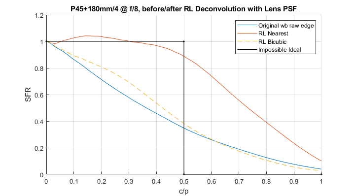
we can take a closer look at each of those components ( $pu$ here indicating normalization to one at the origin). I used Matlab to generate the examples below but you can easily do the same with a spreadsheet. Continue reading A Simple Model for Sharpness in Digital Cameras – Diffraction and Pixel Aperture →

Musings about Photography