Capture Sharpening: Estimating Lens PSF

The next few articles will outline the first tiny few steps towards achieving perfect capture sharpening, that is deconvolution of an image by the Point Spread Function (PSF) of the lens used to capture it. This is admittedly a complex subject, fraught with a myriad ever changing variables even in a lab, let alone in the field. But studying it can give a glimpse of the possibilities and insights into the processes involved.

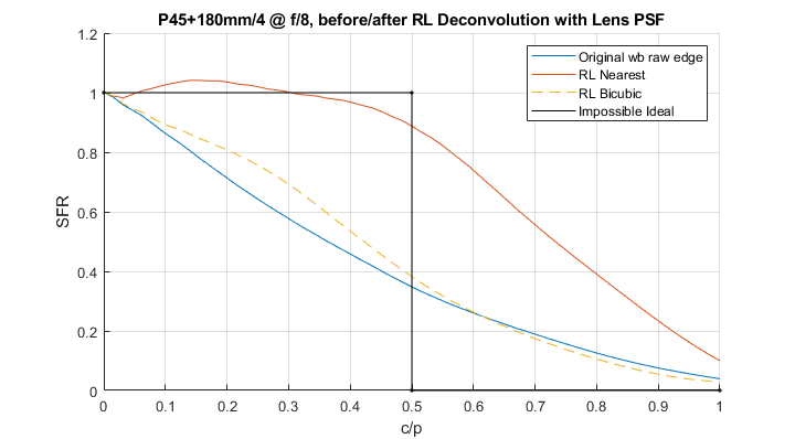
I will explain the steps I followed and show the resulting images and measurements. Jumping the gun, the blue line below represents the starting system Spatial Frequency Response (SFR)^[1], the black one unattainable/undesirable perfection and the orange one the result of part of the process outlined in this series.

Figure 1. Spatial Frequency Response of the imaging system before and after Richardson-Lucy deconvolution by the PSF of the lens that captured the original image.

O Lens PSF, Lens PSF, Wherefore Art Thou Lens PSF?

Wading into the fascinating subject of spatial frequency response of photographic equipment one soon is confronted with the realization that it would be really useful to know the system’s Point Spread Function and its components. But that such PSFs are typically not known.

The system’s point spread function is the cumulative blurring introduced by the hardware during the image capturing process. If one were able to reverse that blurring one would have a perfectly capture-sharpened image, that is an image without the spatial resolution penalties originated within the imaging system itself.

This article will show that in (very) controlled conditions it is possible to estimate the PSF of the lens and use it to undo the blurring that it contributed thus obtaining a ‘perfectly’ capture-sharpened image. This is the first time I attempt such a feat, so think of it as an initial, rudimentary proof of concept.

Simple System PSF = Lens ** Pixel

The system PSF is itself made up of a large number of individual PSF components convolved together: for instance blur introduced by the lens, effective pixel aperture, camera vibration, demosaicing etc. Since we are concentrating on the hardware we are not even going to consider other sources of blur like subject motion, atmospheric turbulence or aerosol scattering.

In fact to keep things simple we are going to assume images obtained from an AA-less sensor, on a tripod, with no vibration, captured and rendered with perfect technique. That effectively leaves only two main sources of blur to discuss: the lens and the pixel aperture (aka footprint) PSFs, as described earlier.

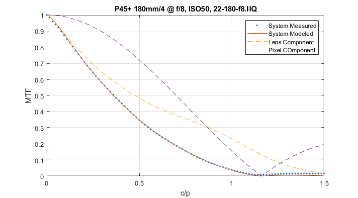
The individual component PSFs are convolved together to obtain the system PSF. The normalized magnitude of the Fourier Transform of a PSF is its Modulation Transfer Function (MTF). Shown below are the MTFs of the Lens and Pixel individually (dashed lines). Convolution in the spatial domain is multiplication in the frequency domain so the system MTF in the plot below (solid curve) is the frequency-by-frequency product of the two dashed component MTFs.

Figure 2. MTF of the indicated system and its main components: Lens and Pixel Aperture. The units are cycles per P45+ pixels, with a pitch of about 6.76 microns.

Reversing the effects of blurring introduced by a PSF is accomplished by deconvolving that PSF from the captured image. Deconvolution in the spatial domain is division in the frequency domain, as better explained here.

For instance, in its simplest form, deconvolving the lens PSF from the capture represented in Figure 2 above would mean dividing the System curve by the Lens curve frequency-by-frequency. The result should be a sharpened image MTF similar to the MTF of pixel aperture alone (we are assuming that the system MTF is the product of the Lens and Pixel MTFs only after all).

The additional energy below the Nyquist frequency (0.5 c/p) introduced by deconvolution is what we are after: that’s all additional ‘sharpness’. However deconvolution also boosts energy above Nyquist – resulting in more aliasing and noise: at some point one will want to filter some of that higher frequency energy out to curtail the amplification of such artifacts in the sharpened image.

Determining Lens PSF

The number of variables involved in accurately determining Lens PSF in a given situation is mind boggling, so achieving perfection is virtually impossible in non-lab conditions – and even then.

For instance some of the variables change with distance, the direction of detail and position in the field of view – so what works in the center of an image may not work at all near its edges. In fact, the use of a single compromise PSF may end up doing more damage than good. For this proof of concept we will therefore concentrate on the center of the field of view, where a decent in-spec prime lens is expected to produce minimal, rotationally symmetric PSFs due mainly to defocus and third order spherical aberrations.

Recall that such aberrations can be described by two Seidel parameters, peak-to-valley Optical Path Difference $W_{020}$ and $W_{040}$ . Or equivalently Zernike polynomial coefficients Z3 and Z8, per Wyant’s notation^[2].

Jack the Knife

In order to obtain these parameters for the lens in question Erik Kaffehr, a fellow traveler in the journey of photographic science discovery, took a set of through-focus captures of a back-lit knife edge near the center of the image, about 3m away, with his Hasselblad 555/ELD and Phase One P45+ digital back mounting a Sonnar 180mm/4 at f/8. He sent me the raw file with the highest MTF^[3], that is the one at ‘best focus’, allegedly with the combination of the two aberrations that resulted in the least lens blur.

Figure 3. The back-lit knife edge raw image used in this article, captured by a Hasselblad 555/ELD and Phase One P45+ digital back mounting a Sonnar 180mm/4 at f/8, courtesy Erik Kaffehr.

Wonderful and robust MTF Mapper by Frans van den Bergh^[4] then used the slanted edge method to extract the green raw channel system SFR curve from the knife edge in the direction perpendicular to it.

Estimating Lens PSF Parameters

The measured SFR curve was then promptly put through a fitting routine that compared it to one produced by a model assuming a square pixel: it varied effective pixel aperture, Z3 and Z8 coefficients until the modeled curve showed the minimum least square error from measured. The ‘model’ is the simple spatial frequency model described in an earlier article. It resulted in the following MTF fit, the same one also shown in Figure 2.

Figure 3. Simple Model fit to Measured SFR curve results in effective square pixel aperture of 0.862 linear Fill Factor and unnormalized Zernike coefficients of 6.0 and 78.8 nm for Z3 and Z8 respectively.

It’s a good fit. The relative parameters are unnormalized Z3 coefficient of 6nm and Z8 of 78.8nm, which for our purposes are interchangeable with peak to valley optical path differences of -0.8804 $\lambda$ and 0.9019 $\lambda$ for $W_{020}$ and $W_{040}$ respectively. I don’t know how realistic these values are in practice but at this stage all we care about is the fact that they describe a lens PSF that results in a good system MTF fit. For what it’s worth I’ve seen Z8 of around 100nm (45nm rms) at f/8 in other lenses online^[5].

This is what the MTF of a lens with those parameters looks like by itself compared to a diffraction limited, circular aperture lens at f/8:

Figure 4. MTF of a lens at f/8 with Z3 coefficient 6nm and Z8 78.8nm, compared to a diffraction limited lens with a circular aperture, also at f/8. Pixels are 6.76 microns apart.

A Radial Slice of the Lens PSF

With those values in hand we can generate a radial slice of the 2D lens PSF thanks to the formula discussed in the article on spherical aberration, which of course is the same formula used by the fitting routine (refer to that article for a description of the variables)^[6]

(1) $\begin{equation*} PSF_{lens}(r) = \frac{P\pi}{(\lambda N)^2}\left|\int_{0}^{1}\gamma(\rho)\cdot J_0 \left[\frac{\pi r}{\lambda N}\rho\right]\cdot \rho \cdot d\rho\right| ^2 \end{equation*}$

with $\gamma(\rho)$ representing the following function when just defocus and third order SA are present

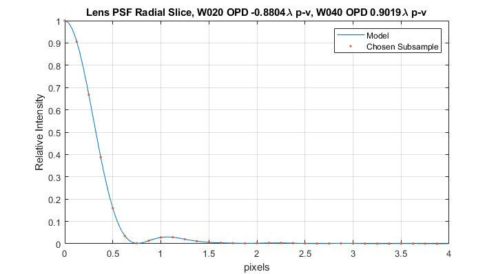
(2) $\begin{equation*} \gamma(\rho) = e^{i\frac{2\pi}{\lambda}(W_{040}\rho^4+W_{020}\rho^2)} \end{equation*}$

This is what the PSF slice looks like with the given $W_{020}$ = -0.8804 $\lambda$ and $W_{040}$ = 0.9019 $\lambda$ ^[7]parameters. The radial axis units are P45+ pixels (pixel pitch = 6.76 microns).

Figure 5. Radial slice of Lens PSF at f/8 with Seidel aberrations of the shown strength.

Rotating the Slice to Produce the 2D Lens PSF

It is obvious that there is a lot of sub-pixel detail in the intensity of this lens PSF. If we were to integrate it over whole pixels we would lose much information to averaging, which would then result in relatively large errors. So I decided to sub-sample PSF intensity at an arbitrary eight times per pixel in order to get a modicum of shape, as shown by the red dots.

In addition, the Bessel function in Equation 1 tells us that this PSF has infinite support – but Figure 5 shows that its intensity decays quickly, so I decided to cut it off at a four pixel radius, per the plot.

Both of these choices affect the size of the PSF that will be used in deconvolution: the larger it is the slower the process, so choices are dictated by a practical trade-off between precision and speed^[8].

To produce the official 2D lens PSF below all we need to do is rotate the generating function, our slice, through 360 degrees. We can do that because both defocus and third order spherical aberrations are rotationally symmetric^[7].

Figure 6. 8x subsampled Lens PSF, f/8, at the given W020 and W040 OPDs

The 2D lens PSF in Figure 6 above has a diameter of 64 samples (a radius of 4 pixels subsampled 8 times). It will need to be normalized so that its area is unity before being put to use.

Putting it to use is the subject of the next article.

Notes and References

_{1. SFR and MTF are used interchangeably in photography. In these pages I tend to use SFR (Spatial Frequency Response) for measured data and MTF (Modulation Transfer Function) for the result of analytical or numerical models.

2. See Wyant and Creath’s Zernike pages for how Seidel and Zernike coefficients are directly related.

3. Thanks to Erik Kaffehr for making his captures available.

4. You can find excellent MTF Mapper here and Frans van den Bergh’s blog here.

5. See the example on this page for a lens at f/8 with Z8 coefficient of 0.175973 * 550 = 96.8nm.

6. Basic Wavefront Aberration Theory for Optical Metrology, James C. Wyant and Katherine Creath.

7. The Matlab/Octave scripts used to generate the PSF can be downloaded from here.

8. In hindsight it would seem that 4x subsampling and a radius of 3 pixels would probably have sufficed, resulting in a lens PSF footprint seven times smaller than the one eventually used.}

Strolls with my Dog