Dynamic Range (DR) in Photography usually refers to the linear working signal range, from darkest to brightest, that the imaging system is capable of capturing and/or displaying.  It is expressed as a ratio, in stops:

   

It is a key Image Quality metric because photography is all about contrast, and dynamic range limits the range of recordable/ displayable tones.  Different components in the imaging system have different working dynamic ranges and the system DR is equal to the dynamic range of the weakest performer in the chain.

Maximum Signal: Easy to Determine

When determining DR for a sensor in a digital still camera the Maximum Acceptable Signal is usually easy to determine quantitatively: it is the photoelectron count or raw level at which a sensor saturates or clips.  The sensor is assumed to behave linearly in its working range.

Minimum Signal: Application Specific

Determining the Minimum Acceptable Signal is a little more subjective and application specific.  The signal is lowered until its quality is at the threshold of becoming unacceptable for the user’s purposes, for instance when its ratio to noise drops below a certain threshold.  Engineers often use an SNR of 1 as a criterion for acceptability;  depending on viewing conditions, photographers would typically find tone quality unacceptable before reaching such a level of noise, so there may be better criteria to determine the minimum signal for their purposes (see for instance Bill Claff’s criteria for Photographic Dynamic Range).  Astrophotographers find signals with an SNR less than one acceptable.  Etc.

Minimum Signal: Not zero (or necessarily 1)

The condition for acceptability always occurs before the signal itself reaches zero, otherwise DR would always be infinite and meaningless.  Nor is a seemingly intuitive integer value of 1 DN (LSB) necessarily the signal’s  lower limit.

Recall from the article on Information Theory definitions that the Signal is the mean output of a limited number of pixels in a uniform region of interest (the sample), so its value is not necessarily an integer: for instance if the sample under investigation is a patch of 20 pixels, all zero except for one with a value of 1 DN, the mean Signal is 0.05 DN.  Therefore the lower bound for the Signal is not a hard number as it usually is for the highlights but it can be a fraction of DN expressed in floating point notation, like SNR.

Engineering Dynamic Range

So Engineering Dynamic Range (eDR) for a photographic sensor is typically expressed in stops and defined as:

   

For instance we could look at DxO average Full SNR curve data for the Canon 7DII at base ISO, realize that  the Signal at which SNR=1 occurs at 0.045% of full scale and conclude that its eDR is log2 of that, or about 11.1 stops, as confirmed by the relative DxO DR chart in ‘screen’ mode.  But what if we do not know the Signal at which SNR=1, what if we only have read noise as is sometimes the case?

How to Get Minimum Signal from Read Noise in e-

Let’s take a closer look at the determinants of SNR.  Our sensor model suggests that

   

with S the mean signal and N total noise standard deviation from a uniform patch in the raw data, r random read noise and g gain.  Upper case letters in units of DN, lower case letters in units of photoelectrons (e-) and g in DN/e-.   In the deepest shadows the PRNU term () is very small compared to the rest so it can be ignored. Substituting 1 for SNR in the formula above we obtain a simple quadratic equation for the Signal when SNR is equal to 1 with two solutions, only one of which works:

(1)  

with signal (s) and random read noise (r) both in units of e-.

An Approximation: Clipping divided by Read Noise

It’s easy to see from equation (1) that if r is more than a few photoelectrons the Signal at which SNR=1 is simply read noise plus half an e-, or approximately just equal to the read noise . Therefore eDR is sometimes approximated by  the ratio of clipping to read noise.  This is how now defunct sensorgen calculated DR using DxO’s data, with the 7DII’s saturation of 29554 divided by a read noise of 12.9 e- producing a DR of 11.2 stops at base ISO.  Close enough to the 11.1 seen earlier.

This approximation however becomes less precise as read noise approaches zero.  For instance at ISO3200 the 7DII’s read noise is about 2.1e-, with saturation at 1236e-.  Sensorgen therefore reported a DR of stops – against DxO’s 8.86, a not inconsequential third of a stop difference.

Applying formula (1) above we can obtain the correct value for the denominator, the signal at which SNR is 1 = 2.66e-, which yields the engineering DR value shown by DxO, 8.86 stops.

Clearly using read noise in the denominator of the formula always results in a higher value for DR than if the Signal at which SNR is equal to one is used, as shown in stops in the graph below:

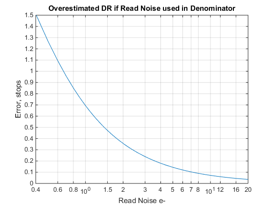
The difference can be quite substantial with cleaner sensors.  For instance with a read noise of 1 e-, using read noise in the denominator will result in a DR 0.7 stops higher than if the Signal @SNR=1 is used.  This level of read noise is not unheard of in current sensors.

What if I have Read Noise in DN/ADU?

In order to perform the same exercise starting with data in units of Data Numbers (also known as Analog to Digital Units) one also needs to know gain (g) in DN/e- for the given ISO.   Solving once more the simple quadratic equation we get

(2)  

with mean Signal (S) and read noise (R) in DN.  eDR is then correctly estimated dividing the clipping raw value by the Signal .  Note that equation (1) is simply equation (2) with gain equal to 1 (thanks Bill for pointing this out).

For instance, Nikon D610 ISO 800 raw file DSC_1569.NEF at dpreview.com shows average read noise in the optical black pixels of 4.63DN and clipping at 15,782DN, which would yield a DR of 11.73  stops with the approximate formula. Sensorgen showed saturation of 9533e- and read noise 2.9e- for a DR of 11.69 stops fitting DxO full SNR curve data, the slight difference  probably due to the fact that the optical pixel read noise data is from a different camera and/or to the different methodologies used.

From this we can estimate average gain as 15782/9533 = 1.655 DN/e- and plug it into formula (2):

   

resulting in an engineering DR of stops.  DxO’s full SNR curves for the D610 show an SNR=1 intercept of 0.036% at ISO800, or an eDR of 11.44 stops, the same small difference as earlier.