Wavefront to PSF to MTF: Physical Units

In the last article we saw that the intensity Point Spread Function and the Modulation Transfer Function of a lens could be easily approximated numerically by applying Discrete Fourier Transforms to its generalized exit pupil function $\mathcal{P}$ twice in sequence.^[1]

Obtaining the 2D DFTs is easy: simply feed MxN numbers representing the two dimensional complex image of the Exit Pupil function in its $uv$ space to a Fast Fourier Transform routine and, presto, it produces MxN numbers representing the amplitude of the PSF on the $xy$ sensing plane. Figure 1a shows a simple case where pupil function $\mathcal{P}$ is a uniform disk representing the circular aperture of a perfect lens with MxN = 1024×1024. Figure 1b is the resulting intensity PSF.

Figure 1a, left: A circular array of ones appearing as a white disk on a black background, representing a circular aperture. Figure 1b, right: Array of numbers representing the PSF of image 1a in the classic shape of an Airy Pattern. — Figure 1. 1a Left: Array of numbers representing a circular aperture (zeros for black and ones for white). 1b Right: Array of numbers representing the PSF of image 1a (contrast slightly boosted).

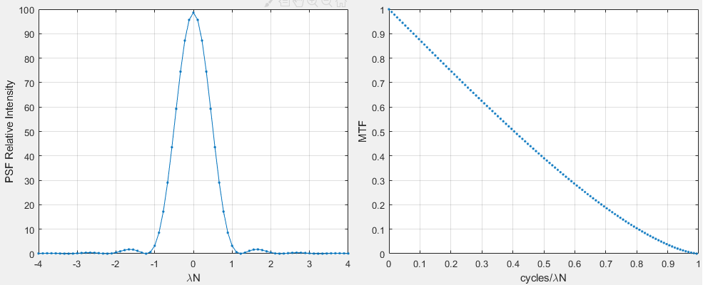
Simple and fast. Wonderful. Below is a slice through the center, the 513th row, zoomed in. Hmm…. What are the physical units on the axes of displayed data produced by the DFT?

Central slice of unaberrated circular aperture DFT, showing the outline of an Airy Pattern — Figure 2. A slice through the center of the PSF shown in figure 1b.

Less easy – and the subject of this article as seen from the point of view of a photographer.

A Numerical Perspective

For this discussion we take a numerical view of Fourier Optics and its black box model of lenses as fully described by their virtual terminal properties, the entrance and exit pupils.^[2] Figure 3 below shows a simplified diagram representing the exit pupil and sensing plane separated by air (not to scale).

The exit pupil function $\mathcal{P}(u,v)$ in this article refers to an array of MxN numbers indexed by integers $u$ and $v$ , which range from 0 to M-1 and 0 to N-1 vertically and horizontally respectively. Similarly for the image of the relative Point Spread Function on the sensing plane $I(x,y)$ and Modulation Transfer Function $MTF(f_x,f_y)$ . The only physical parameters on the diagram are shown in red: exit pupil circular aperture diameter $D$ , focal length $f$ , number of horizontal samples $n$ and sampling pitch $du$ and $dx$ (not shown $dv$ and $dy$ in the vertical direction which would however be the same size as $du$ and $dx$ resp. in a square-pixel sensor).

Figure 3. Simplified representation of the air filled space between the exit pupil of the lens and the image plane, not to scale.

The Physical Units of the Exit Pupil Function

To get the axes of the PSF we first have to determine the physical units of the exit pupil function $\mathcal{P}(u,v)$ , which fortunately we do have because the two domains are linked by a virtual physical window, the aperture. Using the same example as in the last article, with the diameter of the circular aperture $D$ at 5mm, we can easily put axes on Figure 1a above since I counted that exactly 9 diameters fit within a width and a height of the exit pupil image^[3]. That means that in this case the effective MxN $uv$ pupil space related to the MxN $xy$ sensing space must represent a 45mmx45mm physical area.

If the planes are sampled evenly $n$ times in the horizontal direction, with $n$ = N = 1024 per Figure 1, that means that linear physical sample spacing $du$ is 45mm/1024 = 0.0439mm on the physical pupil plane.

Following that reasoning, and denoting the number of times the diameter of the aperture fits horizontally within the pupil plane as $Q$ (a quantization/padding factor, as described in the appendix), the horizontal axis of the pupil function $P(u,v)$ in Figure 1a at index position $u$ would then correspond to physical value

(1) $\begin{equation*} \begin{aligned} u \cdot \frac{QD}{n} \text{ , with u = 0, 1, 2, 3 ...$n$-1} , \\ u \in \mathbb{Z} \end{aligned} \end{equation*}$

and the spacing between samples to $du = \frac{QD}{n}$ , all in the same physical units as $D$ since $Q$ and $n$ are dimensionless. $\mathbb{Z}$ in this case represents integers 0,1,2… to n-1.

That’s with the origin top left, as shown in Figure 1. The convention is however to put the origin of the pupil function $P(0,0)$ in the center of the image as shown in Figure 3. To show an index of zero in the center of the image index $u$ must run from -512 to 511 in our example so in general it becomes

$u = -n/2, -n/2+1, -n/2+2, ...n/2-1.$

Index $u$ would then be equal to zero at the 513th column of Figure 1. Of course physical $du$ remains unaffected by a shifting of the index variable. Assuming square pixels, $dv$ is the same as $du$ and physical values for $v$ can be obtained similarly.

From Pupil Function to PSF Units

To generate the image projected on the $xy$ sensing plane $I(x,y)$ we apply Equation (1) from the previous article to Generalized Exit Pupil Function $\mathcal{P}(u,v)$ , accounting for lens aberrations.

When such image intensity is the result of an on-axis unit impulse of monochromatic light at infinity it allows us to drop the averaging and light field terms. The result is then referred to as the system’s intensity Point Spread Function (PSF) and, after performing coordinate substitution

(2) $\begin{equation*} f_u = \frac{x}{\lambda f} \text{ and } f_v = \frac{y}{\lambda f}, \end{equation*}$

the apparently complex equation is in fact seen to just be the magnitude of the Fourier Transform of $\mathcal{P}(u,v)$ squared, with $\lambda$ the wavelength of light and $f$ the distance in air between the parallel exit pupil $uv$ and sensing $xy$ planes in Figure 3 above, equal to nominal focal length when the lens has unity pupil magnification and is focused at infinity^[iv].

Since in digital photography our unitless MxN data is digitized with samples at regular intervals we can use the Discrete Fourier Transform to approximate the transformation numerically. Here then is the PSF expressed as the DFT of $\mathcal{P}$ with the variables at hand, fixed factors dropped because the PSF and subsequent MTF are otherwise typically normalized by convention depending on the application:^[4]

(3) $\begin{equation*} \begin{aligned} PSF(f_u,f_v) = \left|\sum\limits_{u=0}^{\text{N}-1} \sum\limits_{v=0}^{\text{M}-1} \mathcal{P}(u,v) \cdot e^{-2\pi i(f_u u/\text{N}+ f_v v/\text{M})}\right|^2 \\ f_u,f_v,u,v,\text{N},\text{M} \in \mathbb{Z} \end{aligned} \end{equation*}$

$\mathbb{Z}$ in this case represents integers 0,1,2… to N-1 and M-1 for $u, f_u$ and $v, f_v$ , the coordinates of all the samples in the Pupil and Sensing planes respectively. Of course on the sensing plane each coordinate in the MxN grid corresponds to the center of a physical pixel.

The Discrete Fourier Transform produces an output data set of the same size as the input MxN data set, regardless of any known physical dimensions. Recall that in this case the units produced by the DFT are integers per input set – and the input set refers to the physical extent of the exit pupil function, of length $QD$ on the side. Therefore the horizontal axis of the PSF in Figure 1b at integer index position $f_u$ would correspond to physical value

$f_u \cdot \frac{1}{QD} \text{ , with $f_u$ = 0, 1, 2, 3 ... $n$-1}.$

To convert to units of $x$ on the sensor we simply multiply $f_u$ by $\lambda f$ according to earlier substitution (2) so that, for instance, the fourth pixel on the sensing plane now represents 3 $\frac{\lambda f}{QD}$ in physical units. Substituting effective f-number $N_w$ for $f/D$ in that fraction^[iv]we obtain the following physical value at integer index position $x$ on the horizontal axis of the sensing plane

(4) $\begin{equation*} \begin{aligned} x \cdot \frac{\lambda N_w}{Q} \text{ , with $x$ = 0, 1, 2, 3 ... $n$-1}, \\ x \in \mathbb{Z} \end{aligned} \end{equation*}$

with sample pitch $dx = \frac{\lambda N_w}{Q}$ , all in the same physical units as $\lambda$ because $N_w$ and $Q$ are dimensionless. That’s with the origin top left. If we want the PSF to be centered we shift the origin half an image both ways by changing the index variable ( $x$ this time) as before^[1]:

$x = -n/2, -n/2+1, -n/2+2, ... n/2-1.$

With the origin shifted to the middle of the image, the 513th sample in Figure 2 becomes the origin at index $x$ = 0. It is then easy to see from its central slice that the Airy pattern would hit a first null at $x$ = 11 (count the samples). With $Q$ = 9 this would correspond in physical units to 11/9 $\lambda N$ = 1.22 $\lambda N$ , which is indeed the radius of the first ring predicted by theory.

PSF to MTF Units

To get Modulation Transfer Function $MTF(f_x,f_y)$ from the Point Spread Function we take a second Discrete Fourier Transform of the unitless MxN data, as shown by the third line of code up top. This produces the unnormalized Optical Transfer Function, the normalized modulus of which is the MTF. This time there is no coordinate substitution so the physical units corresponding to the output of the DFT are the bona fide linear spatial frequencies present in the PSF. The physical length of the input set in this case is simply the number of samples $n$ on the $x$ axis times the distance between samples ( $n\cdot dx = \frac{n\lambda N_w}{Q}$ ). Therefore the physical spatial frequencies on the horizontal axis of the relative MTF are obtained by dividing integer index positions $f_x$ by that:

(5) $\begin{equation*} \begin{aligned} f_x \cdot \frac{Q}{n\lambda N_w} \text{ , with $f_x$ = 0, 1, 2, 3 ...$n$-1}, \\ f_x \in \mathbb{Z} \end{aligned} \end{equation*}$

and $df_x = \frac{Q}{n\lambda N_w}$ , all in cycles per the same units as $\lambda$ . Sometimes it is useful to shift the origin of the frequency spectrum to the center of the image. If so proceed as before to also shift index $f_x$ .

Bringing Them All Together

In Octave or Matlab, the three lines of code up top are therefore complemented by the three lines of code below to generate axes for the three planes discussed in this post:

Plots of the pupil, image and frequency spectrum can therefore now be shown with axes in physical units:

Figure 4. Figure 1 and 2 with axes representing physical units.

Units for $y, dy, f_y$ and $df_y$ in the vertical direction can be obtained using the same procedure, this time starting from $dv$ . In the case of Figure 1 they would be exactly the same because both pixel and image are assumed to be square.

Appendix

i) Relating the Physical Pupil and Sensing Planes

With an MxN pixel digital image at hand, and considering the one dimensional case as before for simplicity with N = $n$ , it is clear that since $du = \frac{QD}{n}$ per (1) and $dx = \frac{\lambda f}{QD}$ per (4) sampling pitch in the pupil and sensor domains (hence their relative physical dimensions) are related as follows:

(6) $\begin{equation*} du\cdot dx = \frac{\lambda f}{n} \end{equation*}$

or equivalently in terms of magnification of the image plane vs the pupil plane

(7) $\begin{equation*} \frac{dx\cdot n}{du\cdot n} =\frac{dx}{du} =\frac{\lambda f n}{(QD)^2} \end{equation*}$

In practice as photographers we know $n$ and can typically estimate to a good approximation pixel pitch ( $dx$ ), nominal focal length ( $f$ ) and wavelength ( $\lambda$ ) so Equation (6) provides the easiest link between the two physical planes^[iv].

ii) On Q

You may have noticed that for a given digital image the only variables required to determine the physical units of Exit Pupil, PSF and MTF are light wavelength $\lambda$ , focal length $f$ , exit pupil aperture diameter $D$ – and factor $Q$ , the ratio of the length of the relevant side of the working pupil plane to $D$ .

$Q$ affects the sampling pitch $d_x = \frac{\lambda N_w}{Q}$ in the image plane, with $N_w$ the effective f-number, in a way that can be intuitively related to the size of an Airy Disk. Ignoring rounding errors, there will be about

(8) $\begin{equation*} \frac{1.22\lambda N_w}{d_x} + 1 = 1.22 Q + 1 \text{ samples} \end{equation*}$

from peak intensity to the first zero ring, so in effect it determines how many samples the PSF in the figures will be made up of ( $+1$ because of the sample at the origin, see Figure 5). The larger $Q$ is, the more the PSF samples all else equal. We don’t want $Q$ too small lest we get aliasing in the sensing plane.

Figure 5. PSF and MTF resulting from Figure 1 shown with normalized physical units. Note that with Q = 9 the number of samples between peak PSF intensity and the Airy Disk first zero is 12; and that with n=1024 the relative MTF is made up of about 115 samples between zero and the diffraction extinction spatial frequency.

Following similar thinking in the frequency domain, with $df_x = \frac{Q}{n\lambda N_w}$ and ignoring rounding errors, the MTF curve between zero and the diffraction extinction spatial frequency $\frac{1}{\lambda N_w}$ will be made up of about

(9) $\begin{equation*} \frac{(\lambda N_w)^{-1}}{df_{x}} + 1 = \frac{n}{Q} + 1 \text{ samples} \end{equation*}$

so we don’t want $Q$ too large lest we don’t get enough samples there (Figure 5b), though it’s typically less of an issue here.

Similarly in the pupil plane where $D =\frac{n}{Q}du$ , $Q$ is again in the denominator, which means that the larger $Q$ is the smaller the actual aperture relative to the whole plane and its elements, all else equal – if $Q$ is too large we may get aliasing there.

A happy medium can usually be found for a given total linear number of samples $n$ , as shown in this case with $Q$ = 9 for $n$ = 1024. In some contexts we can think of $Q$ as a padding ratio in the pupil and frequency domains – and a sampling factor in the spatial domain.

iii) On $\lambda N_w$

With $n$ = 1024, a $Q$ value of about one order of magnitude is mainly necessary in order to obtain relatively unaliased data from the Discrete Fast Fourier Transform routines – but for continuous physics photographic thought experiments it can be considered to be equal to one. In that case the physical units of PSFs and MTFs are seen to depend only on a single figure, the product $\lambda N_w$ , as shown for example just above and in figures 2-6 here. This realization can provide some neat insights into the basic properties of light on the sensing plane after it has gone through a lens.

iv) On Working f-number and Macro

The preceding discussion assumes a lens with unity pupil magnification focused at infinity, which places the imaging plane a distance equal to nominal focal length ( $f$ ) from the exit pupil. However it is also valid for most setups including macro if

the size of the region of interest is no greater than about 1/4 the size of the aperture at the exit pupil^[6]
we account for the geometrical change in distance to the imaging plane caused by pupil magnification and/or the focusing plane being other than infinity.

Using Goodman’s notation, in such cases the new distance $z_i$ to the imaging plane replaces $f$ in all equations above (refer to Figure 3). With a little geometric manipulation it can be shown that

(10) $\begin{equation*} z_i = (|m|+p)f \end{equation*}$

with $m$ lens magnification at the given focus distance and $p=D/A$ the ratio of exit ( $D$ ) to entrance ( $A$ ) pupil diameters.^[7] $z_i$ is then the value that becomes the numerator in the calculation of working (or effective) f-number, with the denominator exit pupil aperture diameter $D$ . By definition we can express the latter as the product of pupil magnification $p$ and entrance pupil aperture diameter $A$ , to obtain working f-number $N_w$ ^[8]

(11) $\begin{equation*} N_w = \frac{z_i}{D} = \frac{(|m|+p)}{p}\cdot\frac{f}{A} = (1+\frac{|m|}{p})\codt N \end{equation*}$

where $N$ is the nominal published f-number for the lens focused at infinity. The modifying factor in parentheses preceding it is well known to macro photographers and referred to as the bellows factor. As focus distance increases beyond those of macro photography $m$ becomes increasingly small so $z_i$ tends to $pf$ , the bellows factor tends to 1 and therefore $N_w$ tends to $N$ .

v) On Locality

What about off-axis PSFs? It works the same way as long as one remembers that all results are local to the position of the point source on the sensing plane predicted by geometrical optics.

Lenses perform a 3D transformation. Fourier optics gives us a simplified framework to model the approximate intensity on the sensing plane arising from a point source somewhere in object space – based on the field it produces in the Exit Pupil, represented by the generalized complex pupil function $\mathcal{P}$ .

The position of the pupil within the Exit Pupil plane can be considered to be fixed in this context but the wavefront going through it changes depending on where the point source is located with respect to the lens, on or off axis, closer or further away – and of course so do the relative PSFs, as we all know.

The physical image formed is then the convolution of such a local PSF with the ideal geometric image of the scene projected onto the sensing plane, in the window over which that PSF is valid. Since aberrations vary relatively slowly throughout the field of view it is usually sufficient to produce PSFs at a few (dozen) representative spots for photographic equipment evaluation purposes.

How do we know what Exit Pupil field corresponds to what source position in the scene (hence, by geometrical projection, in the image)? It is up to us to define the wavefront in the Exit Pupil for the point source as set up so that Fourier Optics can perform its magic, as explained below.

vi) On Seidel and Zernike Polynomials

Recall from previous articles that the generalized pupil function $\mathcal{P}(u,v)$ can be expressed in polar coordinates:

(12) $\begin{equation*} \mathcal{P}(\rho,\theta) = e^{2\pi i(polynomial(\rho,\theta))} \end{equation*}$

$\mathcal{P}$ is a map of the complex field in the Exit Pupil plane in polar coordinates, with $\rho$ radial distance of a point from the optical axis and $\theta$ the relative angle. We have already seen this notation in action in the past (for instance here), where the polynomial in the exponent was equal to $W_{040}\rho^4+W_{020}\rho^2$ , with the first term representing the amount of third order Spherical Aberrations present, the second defocus, both in Seidel notation. If coma were also present we would need to add a $W_{131}\rho^3cos\theta$ term – and so on for all additional aberrations.

There are two prevailing aggregations of possible polynomial terms: Seidel and Zernike. Seidel assumes rotational symmetry of the optical surface and concentrates on the more common aberrations, which it gives familiar names like Defocus, Tilt, Spherical Aberrations, Astigmatism, Coma etc., and treats them independently of each other. Zernike instead provides term combinations orthogonal to each other and it is more structured, rigid and complete (careful to be consistent because there are alternative notations in use). You can see a list of two such sets in Wyant^[9], Seidel functionals in Table II and Zernike polynomials in Table III. Each functional/polynomial comes in a certain ‘strength’ represented by its coefficient, what we try to estimate.

vii) Implementation Notes

Practically, to generate a PSF from a lens with a standard circular aperture we could fill a square array with ones, representing a grid of samples of the unaberrated field at the Exit Pupil plane. We would then multiply element by element this pristine wavefront by another array of the same size, populated by values resulting from the complex pupil function $\mathcal{P}(u,v)$ , a result of the aberrations present. Then set all samples outside of the circular pupil to zero to account for the hard stop of the aperture – and let Fourier optics do its job^[*]. Use the discussion on Q in Appendix ii) above as a guide to determine the correct proportions of array size vs aperture diameter (hint: Q needs to be substantially greater than 2). You can see sample code to generate the complex pupil wavefront in Function ‘pupil’ of the attached Matlab class^[5].

Where do the estimated polynomial coefficients come from? Someone has to tell us, or we need to measure them ourselves. See for instance the Appendix in this article for how I estimated the aggregate defocus+SA3 Zernike Z8 coefficient for two of my lenses by using MTF Mapper. Of course those parameters are only valid where measured, in that case on axis, so the resulting PSF is correct just in the center of the sensing plane for a subject at the measured distance. If an estimate of the PSF of that lens in a corner were required, one would need to newly determine Z8 and coefficients for all other relevant aberrations likely present there (e.g. most likely coma, astigmatism, etc. too much work for a curious photographer:). Of course a PSF generated with those parameters would be valid only around there, for a subject at that measured distance.

Notes and References

_{1. The substance of the first line of code above is represented by the two dimensional fast Fourier transform of the Exit Pupil Function (fft2), producing the diffracted pattern on the image plane referred to as the Amplitude Point Spread Function. The shift (fftshift) is there just to make sure that the resulting PSF is centered. The second line is a better and faster way to compute the magnitude squared of the amplitude, which is the intensity PSF. The third line takes the magnitude of the Discrete Fourier Transform of the PSF, which is the MTF of the system. Values are not conventionally normalized.

2. Introduction to Fourier Optics, 3rd Edition. Joseph W Goodman.

3. Simplified Figure 3 is not drawn to scale.

4. The definition of the Discrete Fourier Transform can be found here.

5. If you would like the Matlab routine used to generate these plots let me know via the form available in the ‘About’ page top right. [Edit: I have received enough requests that I have reluctantly decided to make the relative class available. Reluctantly because it was designed to be used just by me (its precursor had contributions by Brandon Dube) so its use is clumsy and non intuitive. You can download it by clicking here.]

6. In Fourier Optics 3rd Edition, Joseph W. Goodman suggests in section 5.3.2 that, in order to drop a quadratic phase factor that depends on object coordinates, the size of the object should be no greater than about one quarter the size of the lens aperture.

7. “Depth of Field from Working F-number and Image magnification“, A Geometric Optics Calculation and comparison with alternative approaches, Alan Robinson (Unpublished, 2020)

8. For a definition of Working f-number see here.

9. Basic Wavefront Aberration Theory for Optical Metrology, James C. Wyant and Katherine Creath.}

2 thoughts on “Wavefront to PSF to MTF: Physical Units”

Raffi says:

November 10, 2022 at 1:57 pm

Thank you for this post. It has been very informative and helpful.

1. Jack says:
  
  November 10, 2022 at 2:39 pm
  
  My pleasure Raffi.
  
  Jack

Strolls with my Dog