The following approach will work if you know the spatial frequency at which a certain MTF relative energy level (e.g. MTF50) is achieved by your camera/lens combination as set up at the time that the capture was taken.

The process by which our hardware captures images and stores them  in the raw data inevitably blurs detail information from the scene.

Even with the best equipment and technique diffraction,  lens blur,  antialiasing filters,  pixel aperture, etc. add up (well, multiply out as we will see)  to degrade our camera system’s spatial resolution ultimate performance –  even before we start processing and rendering images for display.   Attempting to undo some of the blurring inherent in the capture process is the objective of capture sharpening.

The blurring contribution of the main components in a photographic lens/sensor system can be modeled relatively easily in the frequency domain.  The graph below shows how the main hardware components individually attenuate spatial frequency information in our images (dashed lines).  The parameters used are those of a Nikon D4 coupled with a Nikkor 85mm:1.8G at f/5.6.

In the spatial frequency domain the combined effect of more components  is obtained by multiplying their values together.  Doing so produces the overall lens/camera system spatial frequency response (aka MTF curve) shown as the solid black line below.

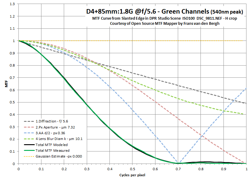
The solid green line is the actual MTF curve for the D4+85mm:1.8G as measured off the slanted edge in the referenced raw file by MTF Mapper, the excellent open source MTF analyzer by Frans van den Bergh.  You can download the raw file  from dpreview.  As you can see theory seems to fit practice fairly well in this case.

Ideally, to undo blurring introduced during the capture process by the hardware all we would need to do is transform our raw image data to the frequency domain and divide out the combined function which resulted in the Total Modeled MTF curve.  Division in the frequency domain is called deconvolution.

Since in this case the two curves are similar, the result of dividing one by the other should be close to 1 throughout the frequency range, which represents  full  spatial frequency transfer from the scene to the raw file.  Hardware blurring undone then,  mission accomplished!

Not so fast.  For a number of reasons, including the fact that every division in the frequency domain can increase noise exponentially, that’s easier said than done.

There is a rough shortcut, however.  The Central Limit Theorem says that the more components contribute to the degradation of the system’s spatial frequency response, the more the system’s Total MTF curve starts to look Gaussian – independently of how the individual component MTF curves look like.  So how close is the D4+85mm:1.8G Total MTF curve to Gaussian for the given set up?  You can see both curves plotted below, the Gaussian is shown as a yellow dotted line and is relative to a PSF of 0.65 pixel standard deviation (radius).

Not a bad fit for the D4+85mm:1.8G at f/5.6.  If we divide (deconvolve) the system’s MTF Total Measured curve by the Gaussian’s the resulting image should in theory show the following MTF spatial frequency response:

Recall that if we ideally had full transfer of all spatial frequencies from the scene to the image recorded in the raw data the Total MTF curve would be a straight line with a value of 1 throughout the range (well, Shannon-Nyquist say that’s impossible so ignore for the moment frequencies much above 0.5 cycles/pixel, the subject of another post). The  Gaussian PSF deconvolution at the specified radius is giving us a fairly decent approximation  of just that .

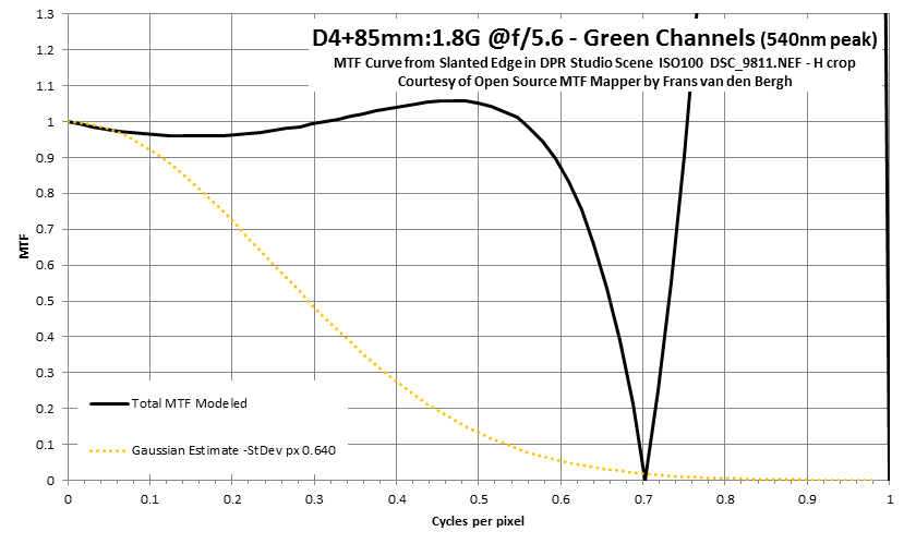
If we had chosen a different radius (standard deviation) for the Gaussian however, things would not have looked as pretty.  Here for instance is a radius of 1 pixel (note the change of vertical scales):

Watch the higher spatial frequencies get amplified through the roof as the Gaussian is no longer a good proxy for system blur and the division produces some seriously unreal results. In addition noise also throws a wrench in ideal deconvolution by division in the frequency domain, as you can see in this article.  Deconvolution plug-in designers resort to iterative techniques and advanced low-pass filters to try to keep noise and the higher frequencies in check, as you can read in the article on Richardson-Lucy deconvolution.

So if we want to stay in the ballpark, how do we choose the radius for deconvolution with a generic Gaussian PSF for a given camera/lens?

If we know the spatial frequency at which a certain MTF relative energy level is achieved in cycles per pixel as set up (e.g. 50% of peak MTF, aka MTF50, at 0.29 c/p), one way is to notice that the D4’s well behaved total MTF curve looks like a reverse S just like a Gaussian.   Let’s then choose a value for the radius/standard deviation of the Gaussian that will make the two curves intersect at the known MTF energy level and spatial frequency.  The Standard Deviation of a Gaussian PSF that will result in MTF level at spatial frequency in cycles per pixel is:

(1)  

For frequencies measured at MTF50 ,  , so

(2)  

In this case half of the Gaussian curve tends to overestimate MTF while the other half underestimates it, refer to Figure 2.

With our example, Figure 1 shows measured MTF50 at =0.29 cycles per pixel for the camera/lens combination as setup, which when plugged into the equation results in a corresponding Gaussian PSF radius of 0.646 pixels (to convert from different units of spatial resolution see this article).

If the camera/lens system is not well behaved, and by that I mean that the Measured System MTF curve is not approximately Gaussian, all bets are off – though as mentioned a Gaussian shape will often be a decent approximation in practice when there are several sources of blur, thanks to the Central Limit Theorem.

That’s  one way to estimate the radius for deconvolution by a Gaussian PSF with well behaved cameras such as the D4 when the MTF50 of the setup is known.  Applying deconvolution with that radius will very roughly attempt to undo  the blurring effects of the hardware during the capture process, what Capture Sharpening is all about – keeping in mind that we have not dealt with blurring introduced by downstream processes like the demosaicing process – and several practical issues linked to noise and insufficient energy in the measured curve. Hopefully the app used for deconvolution will be smart enough to deal with those with aplomb.

Of course if the set up changes so does the radius, as you can read in the next post.